Mechanical Engineering Report: Truss Deflection and Strain Analysis

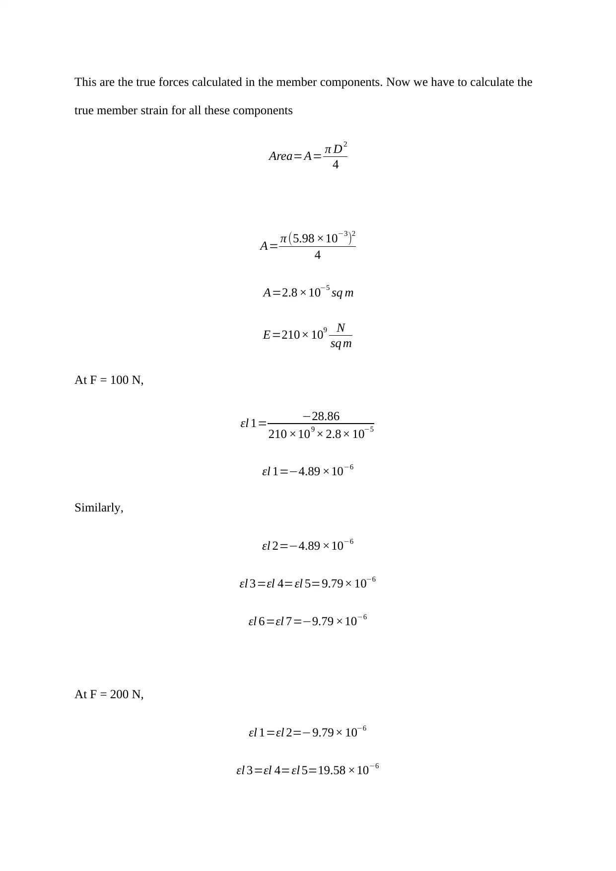
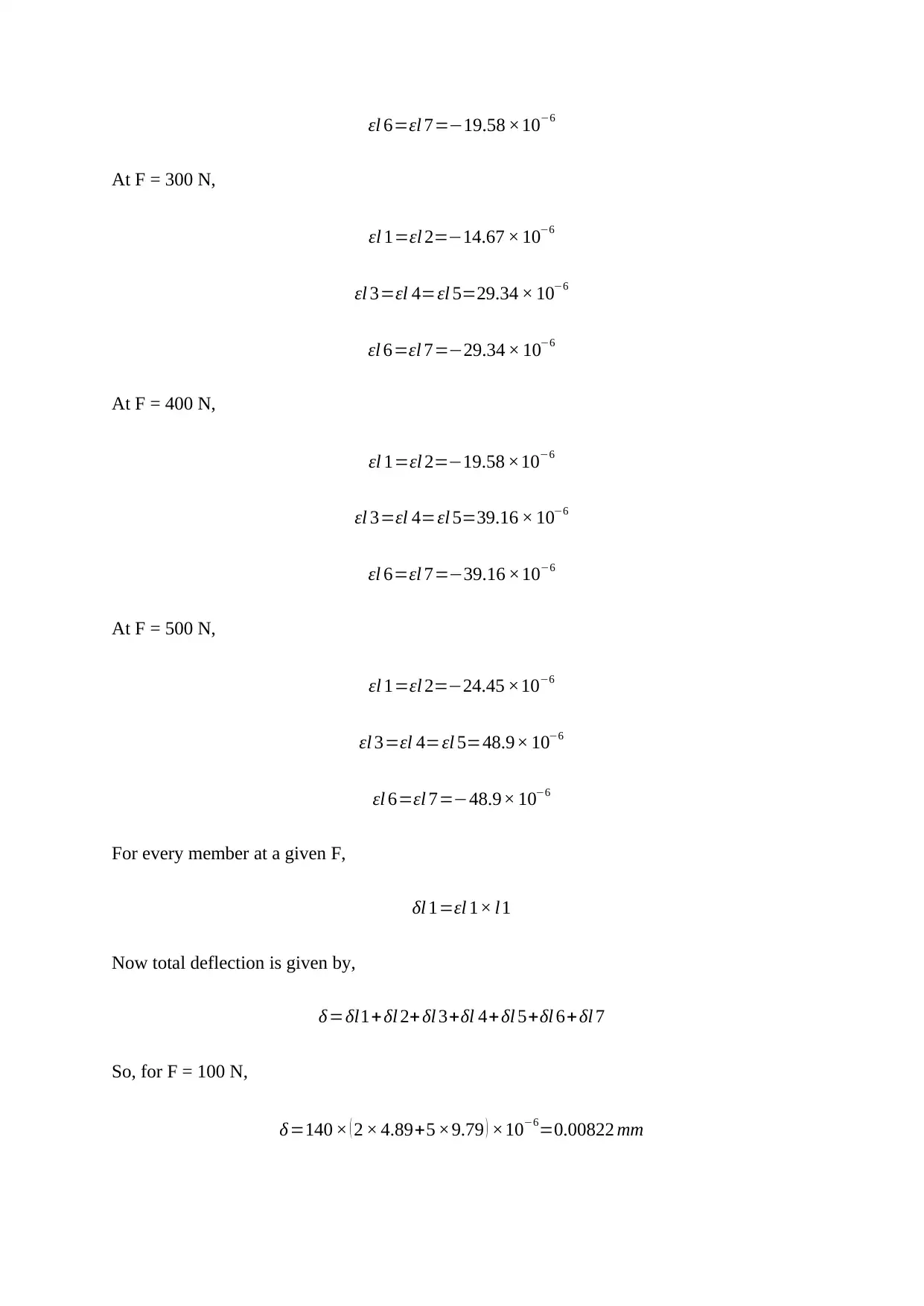
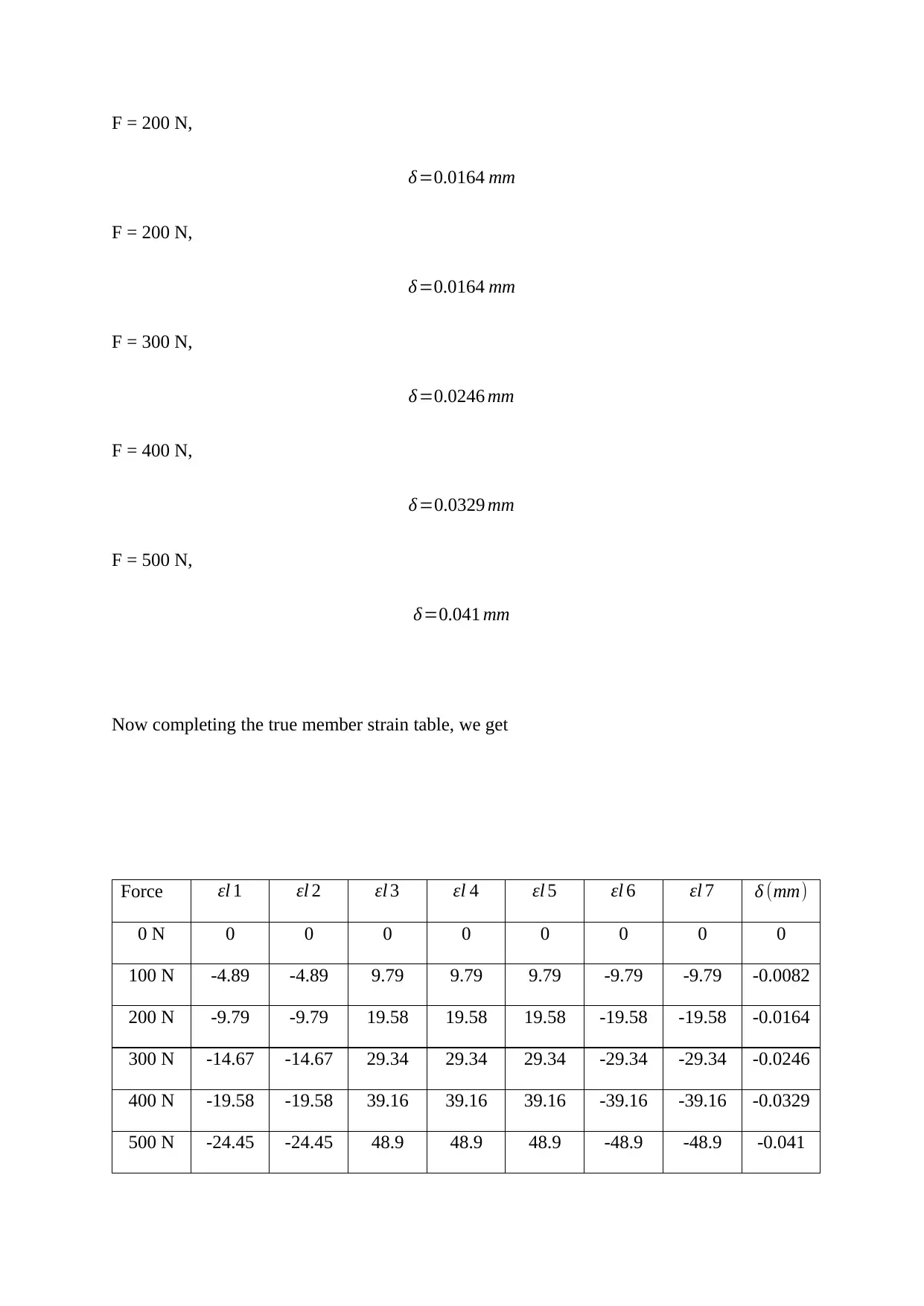
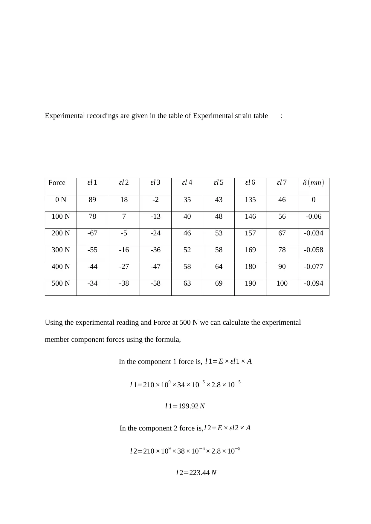
This report presents an analysis of truss deflection, integrating theoretical calculations with experimental results using strain gauges. The experiment focuses on a truss structure, applying the method of joints to determine internal forces within the members. The report details the procedure, including the application of stress-strain equations and Hooke's law to calculate deflection. The results section presents calculated and experimental strain and deflection values for different load scenarios. A discussion of the errors and discrepancies between the theoretical and experimental results is provided, highlighting potential sources of error such as external forces and component variations. The report offers a comprehensive understanding of structural behavior under load and the practical application of strain gauges in civil and mechanical engineering contexts.

INTRODUCTION
In this experiment, it provides a visualisation of the relative deflections of a joint in a
truss. It also demonstrates the basic theory of static equilibrium and understanding how the
structure supports load and how much strain each member can withstand. The experiment
also demonstrates the use of strain gauge. This type of experiment in real life condition is
used to check the sustainability of the bridges and different types of civil construction. We
have considered here a truss and its member forces are calculated using the Method of Joints
and after that applied the stress strain equation to calculate the deflection in the structural
material. All the calculations of this strain and deflection and the force acting can be found
out using different types of formula whose reference is given in the reference section of the
report.
In the initial (low strain) portion of the stress strain curve, almost all the materials
obey Hooke’s law to a some extent where the stress is proportional to strain with the constant
of proportionality called the modulus of elasticity or Young’s modulus, denoted by E.
Increase in the strain, helps the materials to deviate from its linear characteristic and the point
where the departure takes place is known as the proportional limit. The nonlinearity happens
due to the stress-induced “plastic” flow in the specimen. In the plastic flow the material is
undergoing a rearrangement of its internal molecular structure in which the atoms are being
moved to new equilibrium positions. So the atoms becomes mobile in nature and tries to
change the properties of the material. It may happen that the materials lacking this mobility,
which can happen due to blocking of the dislocation motion, are usually found to be brittle
rather than ductile. The stress-strain curve for brittle materials are linear over their full range
of applied force which causes the strain, eventually terminating in fracture mode.to get in to
the plastic flow, stress needed to increase the strain beyond the proportional limit in a ductile

material continues to rise beyond the proportional limit; strain hardening is a term which can
be used in this scenario where the material requires an ever-increasing stress to continue
straining. So once a material goes in to the plastic flow it cannot come back to the original
material condition, so the proportional limit is mostly same as or at least close to the
material’s elastic limit. Elasticity is the property where if we remove the load from the
material then it returns to its original structure and when it is not able to return to its original
structure we can interpret that it went to its plastic mode. In this experiment we are also going
to analyse that whether any components are going to the plastic mode because of the increase
in the loading factor which will show discrepancy in the experimental result. (Roylance,
2001)
PROCEDURE
First we take the deflection of each of the member components of the truss where a
single load is applied on the truss. In the later part we will see how the forces will get
distributed. Now for each member components let the force getting applied is F. (Roorkee,
n.d.)
Then we can write
σ =F / A
Where σ is the stress and A is the area of the member component and when the stress is
applied on the rod, the rod is under some strain which causes deflection
σ =E × ε
Where ε the strain and E is the Young Modulus

Now the strain is defined as the deflection per unit length of the member component
ε =δ / L
Using all the three equations we can write,
F=E × ε × A
 ε =F /E × A
F=E × δ / L× A
Now given the truss diagram let’s calculate the force on each of the member
In the Method of Joints we analyse first the external forces which generally
constitutes the applied force and the reaction force coming from the hinge and the roller.
Once we get the external forces we start finding out the internal forces in each of the member.
To find out the internal force, we consider all the joints where the member component have
been joined and in each joint we sum the forces in the both horizontal direction and vertical
direction to zero. Since the structure is internally stable we do that. Consider the figure
below showing the external force equilibrium and internal force equilibrium at each of the
joints and the corresponding calculations will be done based on this diagram. (Kanpur, n.d.)
Considering the external forces at the hinge and at the roller
Cy + Ay = W (from the force equilibrium in the y axis)
Ax = 0 (from the force equilibrium in the x axis)
Cy × L = Ay × L (from moments equation)
Solving this three equations we get,

Ay = W/2
Cy = W/2
So at the point A the external force is W/2 and at the point C the external force is W/2 and
both the forces are in the upward direction
Now let’s consider the internal forces now,

At the joint B
Considering the force equilibrium in the x axis,
l 7× cos 60+l 1=F l 6 ×cos 60+l2
l 7+2× l1=l6+ 2× l2
Considering the force equilibrium in the y axis,
l 7× sin 60+l 6 ×sin 60=W
l 7+l6=2 × W
√3
At the joint A,
Considering the force equilibrium in the y axis,
l 3× sin 60= W
2
l 3= W
√3
Considering the force equilibrium in the x axis,
l 1=l3 × cos 60
l 1= W
2 √3
At the joint C,
Considering the force equilibrium in the y axis,
l 5× sin 60= W
2

l 5= W
√ 3
Considering the force equilibrium in the x axis,
l 2=l5 × cos 60
l 2= W
2 √ 3
Now putting the value of l 2∧l1 we get,
l 7+ W
√3 =l 6+ W
√3
l 7=l 6
2 ×l7=2 × W
√ 3
l 7= W
√3
l 6= W
√3
At the joint D,
Considering the force equilibrium in the x axis,
l 6 ×cos 60+l 5 ×cos 60+l 4=0
l 4=−W
√ 3
Now the individual final force acting on the members are:

l 1= W
2 √3 (Compression)
l 2= W
2 √3 (Compression)
l 3= W
√3 (Tensile)
l 4= W
√3 (Tensile)
l 5= W
√ 3 (Tensile)
l 6= W
√3 (Compression)
l 7= W
√ 3 (Compression)
RESULT
At W = 0 N,
l 1=l2=l3=l 4=l5=l 6=l 7=0
At W = 100 N
l 1=l2=−28.86 N
l 3=l 4=l 5=57.74 N
l 6=l 7=−57.74 N

At W = 200 N
l 1=l2=−57.74 N
l 3=l 4=l 5=115.47 N
l 6=l 7=−115.47 N
At W = 300 N
l 1=l2=−86.58 N
l 3=l 4=l 5=173.22 N
l 6=l 7=−173.22 N
At W = 400 N
l 1=l2=−115.44 N
l 3=l 4=l 5=230.96 N
l 6=l 7=−230.96 N
At W = 500 N
l 1=l2=−144.3 N
l 3=l 4=l 5=288.7 N
l 6=l 7=−288.7 N

This are the true forces calculated in the member components. Now we have to calculate the
true member strain for all these components
Area=A= π D2
4
A= π (5.98 ×10−3)2
4
A=2.8 ×10−5 sq m
E=210× 109 N
sq m
At F = 100 N,
εl 1= −28.86
210 ×109 × 2.8× 10−5
εl 1=−4.89 ×10−6
Similarly,
εl 2=−4.89 ×10−6
εl 3=εl 4=εl 5=9.79× 10−6
εl 6=εl 7=−9.79 ×10−6
At F = 200 N,
εl 1=εl 2=−9.79× 10−6
εl 3=εl 4=εl 5=19.58 ×10−6

εl 6=εl 7=−19.58 ×10−6
At F = 300 N,
εl 1=εl 2=−14.67 × 10−6
εl 3=εl 4=εl 5=29.34 × 10−6
εl 6=εl 7=−29.34 × 10−6
At F = 400 N,
εl 1=εl 2=−19.58 ×10−6
εl 3=εl 4=εl 5=39.16 × 10−6
εl 6=εl 7=−39.16 ×10−6
At F = 500 N,
εl 1=εl 2=−24.45 ×10−6
εl 3=εl 4=εl 5=48.9× 10−6
εl 6=εl 7=−48.9× 10−6
For every member at a given F,
δl 1=εl 1× l1
Now total deflection is given by,
δ=δl1+ δl 2+ δl 3+δl 4+δl 5+δl 6+ δl 7
So, for F = 100 N,
δ=140 × ( 2 × 4.89+5 ×9.79 ) ×10−6=0.00822 mm

F = 200 N,
δ=0.0164 mm
F = 200 N,
δ=0.0164 mm
F = 300 N,
δ =0.0246 mm
F = 400 N,
δ=0.0329 mm
F = 500 N,
δ=0.041 mm
Now completing the true member strain table, we get
Force εl 1 εl 2 εl 3 εl 4 εl 5 εl 6 εl 7 δ (mm)
0 N 0 0 0 0 0 0 0 0
100 N -4.89 -4.89 9.79 9.79 9.79 -9.79 -9.79 -0.0082
200 N -9.79 -9.79 19.58 19.58 19.58 -19.58 -19.58 -0.0164
300 N -14.67 -14.67 29.34 29.34 29.34 -29.34 -29.34 -0.0246
400 N -19.58 -19.58 39.16 39.16 39.16 -39.16 -39.16 -0.0329
500 N -24.45 -24.45 48.9 48.9 48.9 -48.9 -48.9 -0.041

Experimental recordings are given in the table of Experimental strain table :
Force εl 1 εl 2 εl 3 εl 4 εl 5 εl 6 εl 7 δ (mm)
0 N 89 18 -2 35 43 135 46 0
100 N 78 7 -13 40 48 146 56 -0.06
200 N -67 -5 -24 46 53 157 67 -0.034
300 N -55 -16 -36 52 58 169 78 -0.058
400 N -44 -27 -47 58 64 180 90 -0.077
500 N -34 -38 -58 63 69 190 100 -0.094
Using the experimental reading and Force at 500 N we can calculate the experimental
member component forces using the formula,
In the component 1 force is, l 1=E × εl1 × A
l 1=210 ×109 ×34 × 10−6 ×2.8 ×10−5
l 1=199.92 N
In the component 2 force is,l 2=E × εl2 × A
l 2=210 ×109 ×38 ×10−6 × 2.8 ×10−5
l 2=223.44 N