MEEM 5715 Linear Systems Final Exam Solution: Base Excitation System

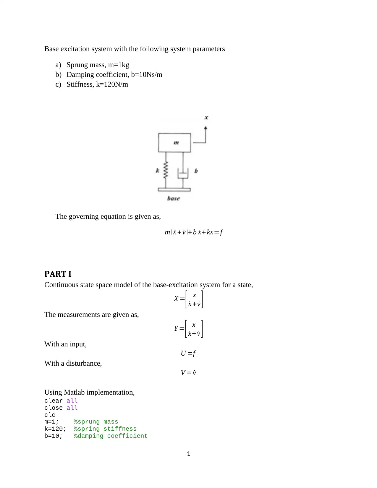
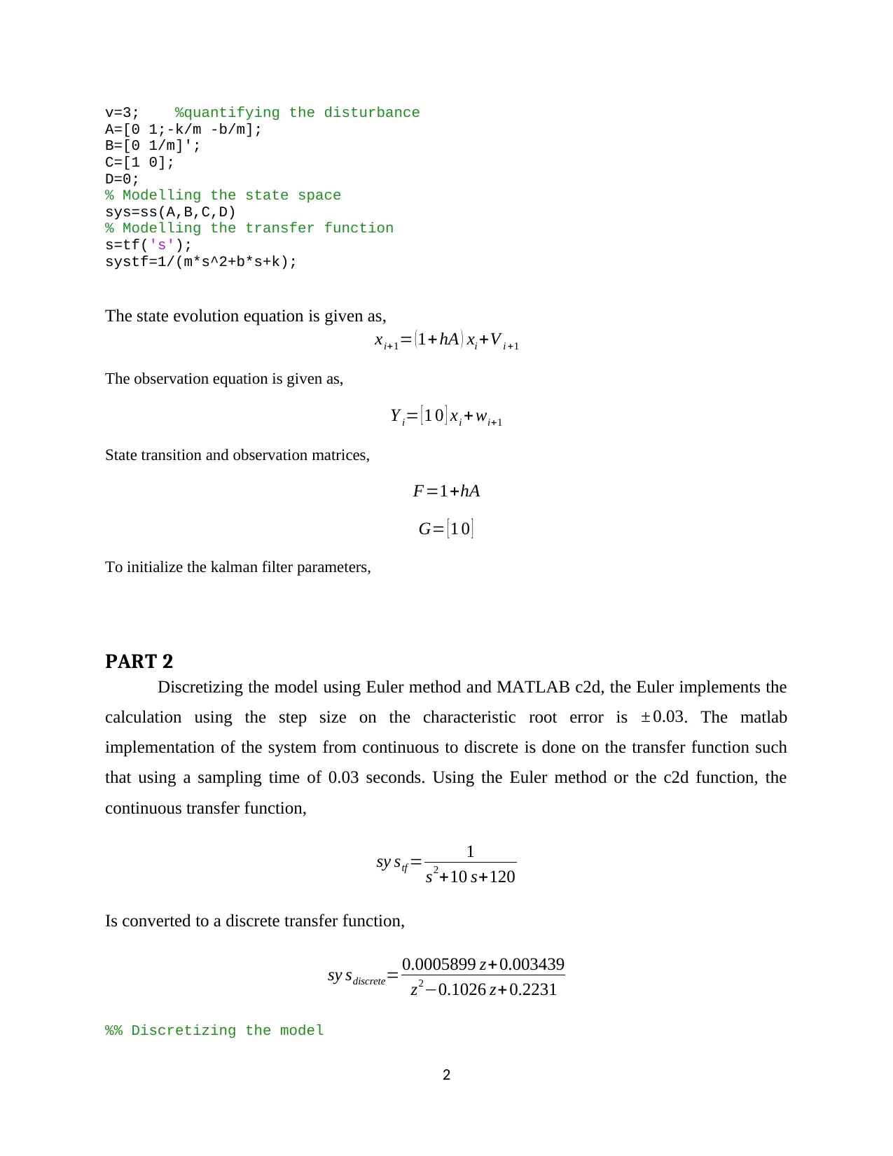
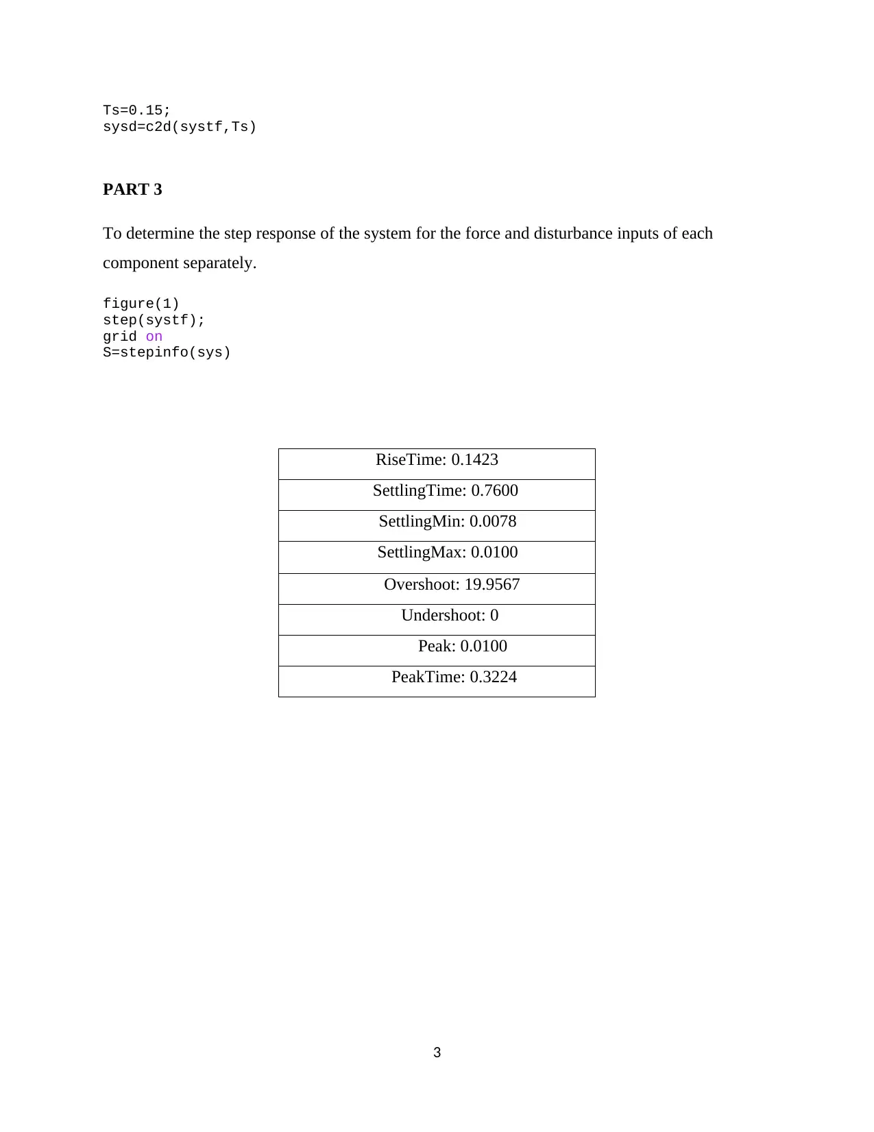
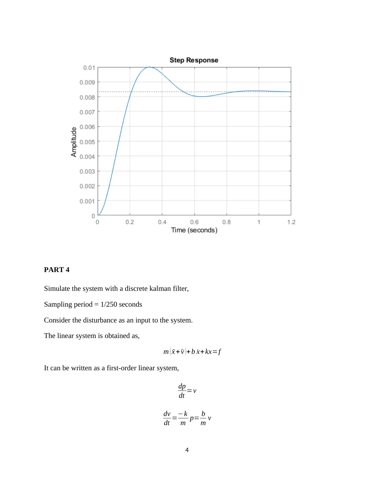
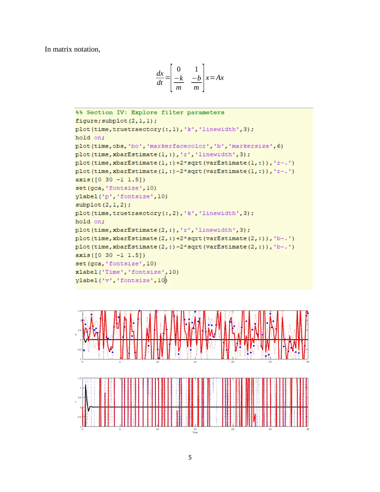
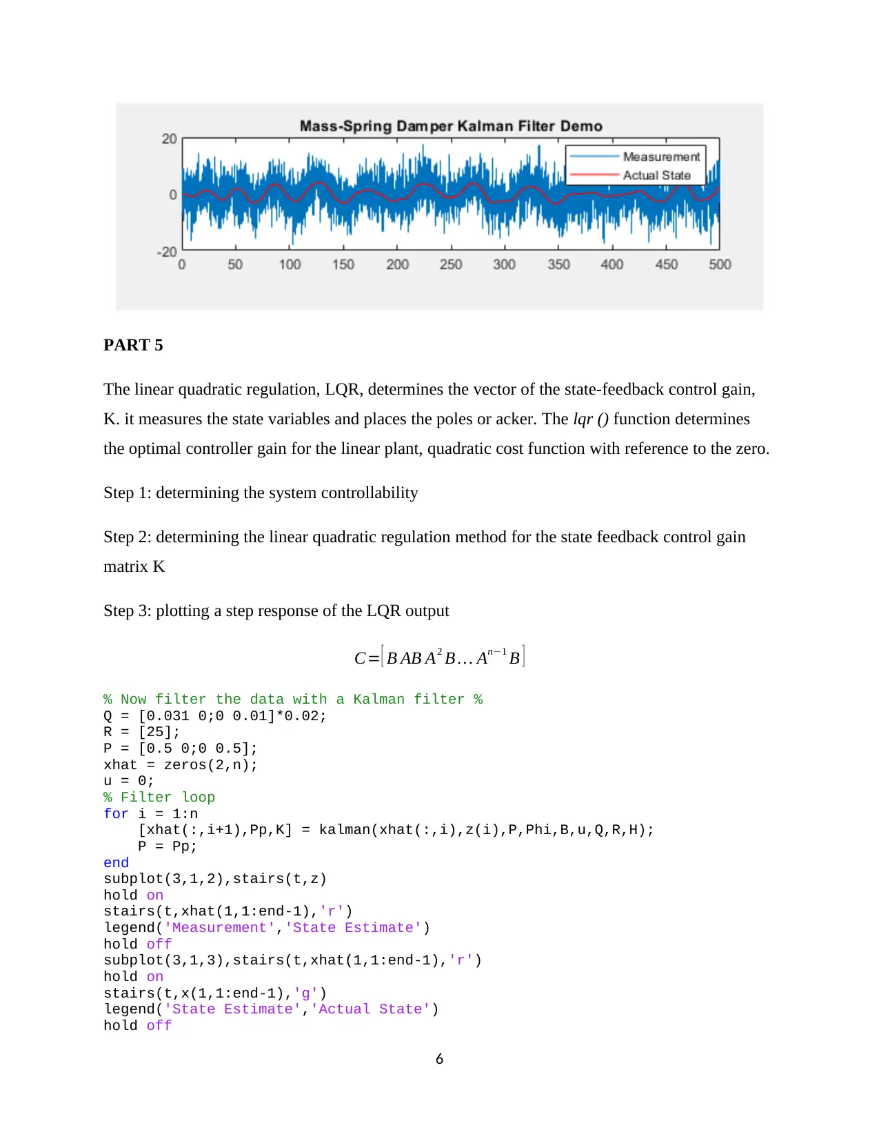
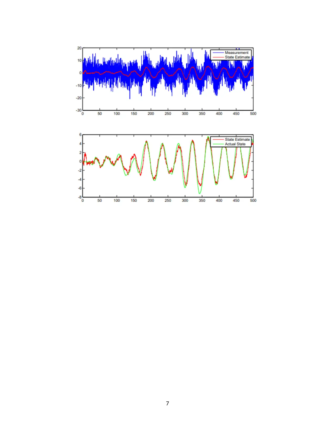
This document presents a comprehensive solution to the MEEM 5715 Linear Systems final exam, focusing on a base excitation system. The solution begins with the continuous state space model, defining system parameters like sprung mass, damping coefficient, and stiffness, and provides the governing equation. It includes MATLAB implementations for state space modeling and transfer function analysis. The solution then covers the discretization of the model using the Euler method and MATLAB's c2d function, converting the continuous transfer function to a discrete one. Step responses for force and disturbance inputs are determined and visualized. The document continues with the simulation of the system using a discrete Kalman filter, outlining the linear system equations and matrix notation. Finally, the linear quadratic regulation (LQR) method is applied to determine the state-feedback control gain and plot the step response of the LQR output. The solution includes detailed explanations, MATLAB code snippets, and graphical representations to facilitate understanding of the concepts and methodologies used.

MEEM 5715 linear Systems
Final exam
Student name
Base Student ID Number
Institutional Affiliation
Date of submission
12/12/2018

Base excitation system with the following system parameters
a) Sprung mass, m=1kg
b) Damping coefficient, b=10Ns/m
c) Stiffness, k=120N/m
The governing equation is given as,
m ( ¨x + ¨v )+ b ˙x+ kx=f
PART I
Continuous state space model of the base-excitation system for a state,
X =
[ x
˙x + ˙v ]
The measurements are given as,
Y = [ x
˙x+ ˙v ]
With an input,
U =f
With a disturbance,
V = ˙v
Using Matlab implementation,
clear all
close all
clc
m=1; %sprung mass
k=120; %spring stiffness
b=10; %damping coefficient
1

v=3; %quantifying the disturbance
A=[0 1;-k/m -b/m];
B=[0 1/m]';
C=[1 0];
D=0;
% Modelling the state space
sys=ss(A,B,C,D)
% Modelling the transfer function
s=tf('s');
systf=1/(m*s^2+b*s+k);
The state evolution equation is given as,
xi+1= ( 1+ hA ) xi +V i +1
The observation equation is given as,
Y i= [ 1 0 ] xi + wi+1
State transition and observation matrices,
F=1+hA
G= [ 1 0 ]
To initialize the kalman filter parameters,
PART 2
Discretizing the model using Euler method and MATLAB c2d, the Euler implements the
calculation using the step size on the characteristic root error is ± 0.03. The matlab
implementation of the system from continuous to discrete is done on the transfer function such
that using a sampling time of 0.03 seconds. Using the Euler method or the c2d function, the
continuous transfer function,
sy stf = 1
s2+10 s+120
Is converted to a discrete transfer function,
sy sdiscrete= 0.0005899 z+ 0.003439
z2−0.1026 z+0.2231
%% Discretizing the model
2

Ts=0.15;
sysd=c2d(systf,Ts)
PART 3
To determine the step response of the system for the force and disturbance inputs of each
component separately.
figure(1)
step(systf);
grid on
S=stepinfo(sys)
RiseTime: 0.1423
SettlingTime: 0.7600
SettlingMin: 0.0078
SettlingMax: 0.0100
Overshoot: 19.9567
Undershoot: 0
Peak: 0.0100
PeakTime: 0.3224
3

PART 4
Simulate the system with a discrete kalman filter,
Sampling period = 1/250 seconds
Consider the disturbance as an input to the system.
The linear system is obtained as,
m ( ¨x + ¨v )+ b ˙x+ kx=f
It can be written as a first-order linear system,
dp
dt =v
dv
dt =−k
m p= b
m v
4

In matrix notation,
dx
dt =
[ 0 1
−k
m
−b
m ] x=Ax
0 5 10 15 20 25 30
-1
-0.5
0
0.5
1
1.5
p
0 5 10 15 20 25 30
Time
-1
-0.5
0
0.5
1
1.5
v
5

PART 5
The linear quadratic regulation, LQR, determines the vector of the state-feedback control gain,
K. it measures the state variables and places the poles or acker. The lqr () function determines
the optimal controller gain for the linear plant, quadratic cost function with reference to the zero.
Step 1: determining the system controllability
Step 2: determining the linear quadratic regulation method for the state feedback control gain
matrix K
Step 3: plotting a step response of the LQR output
C= [ B AB A2 B … An−1 B ]
% Now filter the data with a Kalman filter %
Q = [0.031 0;0 0.01]*0.02;
R = [25];
P = [0.5 0;0 0.5];
xhat = zeros(2,n);
u = 0;
% Filter loop
for i = 1:n
[xhat(:,i+1),Pp,K] = kalman(xhat(:,i),z(i),P,Phi,B,u,Q,R,H);
P = Pp;
end
subplot(3,1,2),stairs(t,z)
hold on
stairs(t,xhat(1,1:end-1),'r')
legend('Measurement','State Estimate')
hold off
subplot(3,1,3),stairs(t,xhat(1,1:end-1),'r')
hold on
stairs(t,x(1,1:end-1),'g')
legend('State Estimate','Actual State')
hold off
6

7