Business Finance Plan: Melbourne Housing Price and Income Analysis

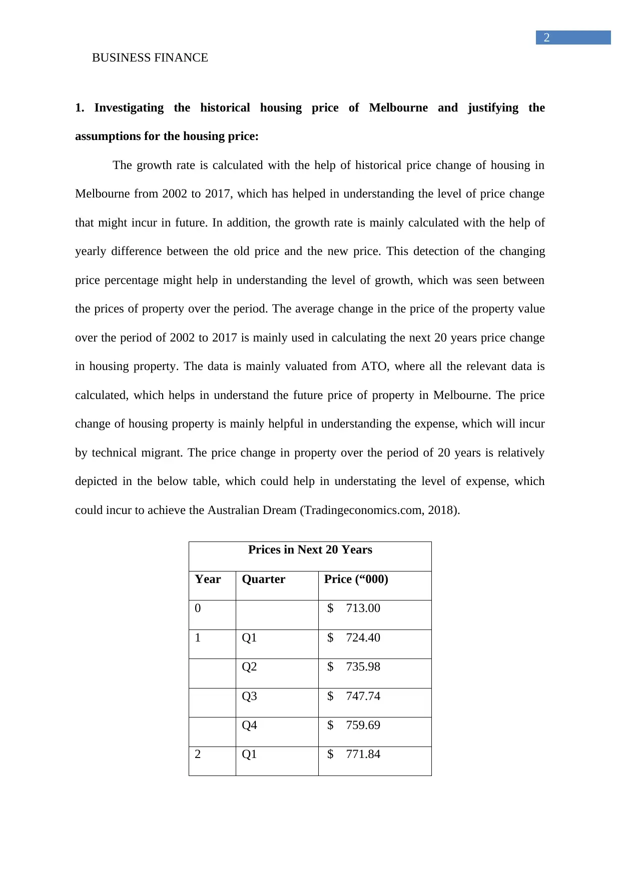
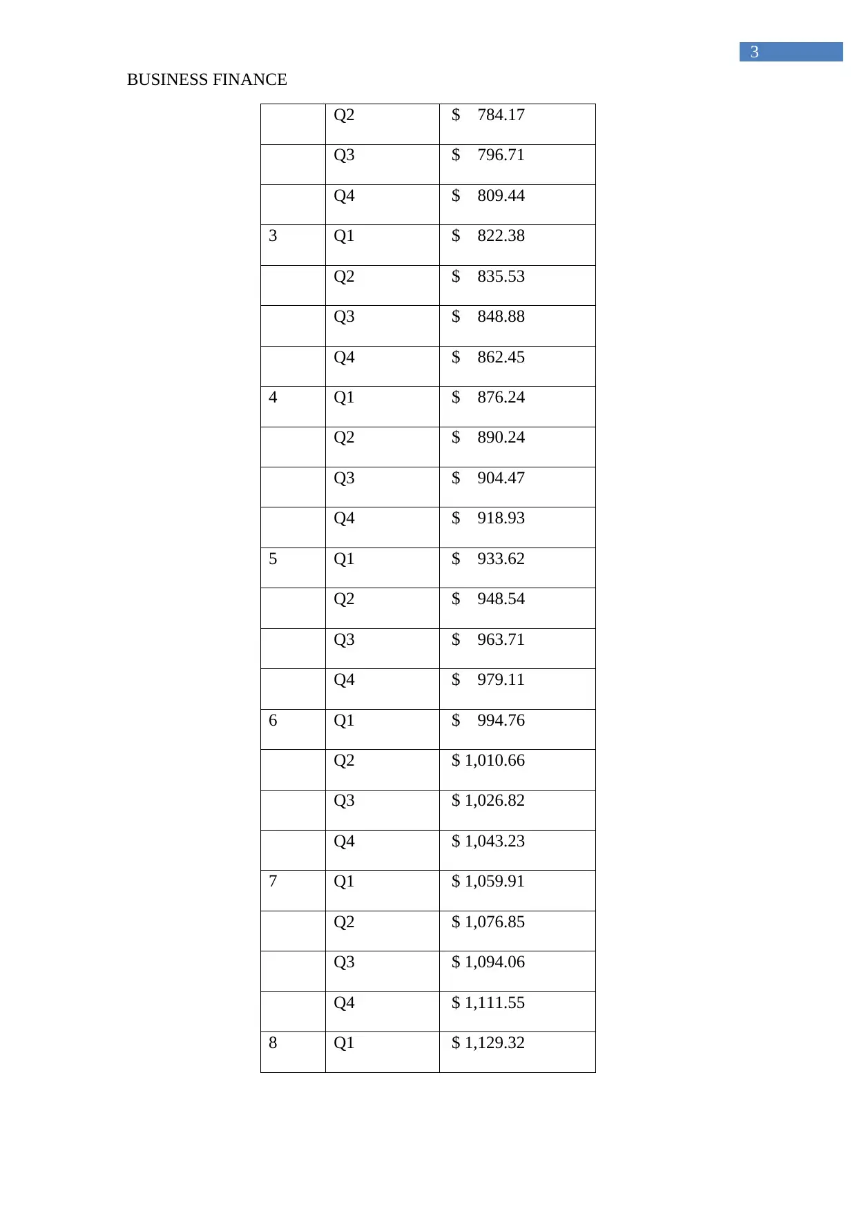
This project presents a business finance plan focused on the Melbourne housing market. It begins by investigating historical housing prices and income data, justifying assumptions made for future projections. The analysis includes calculating net income using the ATO calculator, determining home loa...Read More

Running head: BUSINESS FINANCE
Business Finance
Name of the Student:
Name of the University:
Authors Note:

BUSINESS FINANCE
1
Table of Contents
1. Investigating the historical housing price of Melbourne and justifying the assumptions for
the housing price:.......................................................................................................................2
2. Investigating the historical income data of Melbourne and justifying the assumptions for
the income data:.........................................................................................................................6
3. Calculating the net income by using the ATO calculator, while detecting the home loan
rate and maximum amount it could borrow in current sphere:..................................................8
4. Calculating the stamp duty situated with property purchase, while detecting the house price
client can afford:........................................................................................................................9
5. Drafting the financial Plan where upfront payment of 20% is calculated and 5% upfront
payment in calculated for loan:................................................................................................10
6. Calculating whether increment in interest payment can hamper interest payment capability
of the lender:............................................................................................................................12
7. Providing a relevant plan with detailed risk entailed by the assumption made for the
financial plan:...........................................................................................................................13
Reference and Bibliography:....................................................................................................14

BUSINESS FINANCE
2
1. Investigating the historical housing price of Melbourne and justifying the
assumptions for the housing price:
The growth rate is calculated with the help of historical price change of housing in
Melbourne from 2002 to 2017, which has helped in understanding the level of price change
that might incur in future. In addition, the growth rate is mainly calculated with the help of
yearly difference between the old price and the new price. This detection of the changing
price percentage might help in understanding the level of growth, which was seen between
the prices of property over the period. The average change in the price of the property value
over the period of 2002 to 2017 is mainly used in calculating the next 20 years price change
in housing property. The data is mainly valuated from ATO, where all the relevant data is
calculated, which helps in understand the future price of property in Melbourne. The price
change of housing property is mainly helpful in understanding the expense, which will incur
by technical migrant. The price change in property over the period of 20 years is relatively
depicted in the below table, which could help in understating the level of expense, which
could incur to achieve the Australian Dream (Tradingeconomics.com, 2018).
Prices in Next 20 Years
Year Quarter Price (“000)
0 $ 713.00
1 Q1 $ 724.40
Q2 $ 735.98
Q3 $ 747.74
Q4 $ 759.69
2 Q1 $ 771.84

BUSINESS FINANCE
3
Q2 $ 784.17
Q3 $ 796.71
Q4 $ 809.44
3 Q1 $ 822.38
Q2 $ 835.53
Q3 $ 848.88
Q4 $ 862.45
4 Q1 $ 876.24
Q2 $ 890.24
Q3 $ 904.47
Q4 $ 918.93
5 Q1 $ 933.62
Q2 $ 948.54
Q3 $ 963.71
Q4 $ 979.11
6 Q1 $ 994.76
Q2 $ 1,010.66
Q3 $ 1,026.82
Q4 $ 1,043.23
7 Q1 $ 1,059.91
Q2 $ 1,076.85
Q3 $ 1,094.06
Q4 $ 1,111.55
8 Q1 $ 1,129.32

BUSINESS FINANCE
4
Q2 $ 1,147.37
Q3 $ 1,165.71
Q4 $ 1,184.34
0 Q1 $ 1,203.27
Q2 $ 1,222.51
Q3 $ 1,242.05
Q4 $ 1,261.90
10 Q1 $ 1,282.07
Q2 $ 1,302.57
Q3 $ 1,323.39
Q4 $ 1,344.54
11 Q1 $ 1,366.03
Q2 $ 1,387.87
Q3 $ 1,410.05
Q4 $ 1,432.59
12 Q1 $ 1,455.49
Q2 $ 1,478.76
Q3 $ 1,502.39
Q4 $ 1,526.41
13 Q1 $ 1,550.81
Q2 $ 1,575.60
Q3 $ 1,600.78
Q4 $ 1,626.37
14 Q1 $ 1,652.36

BUSINESS FINANCE
5
Q2 $ 1,678.78
Q3 $ 1,705.61
Q4 $ 1,732.88
15 Q1 $ 1,760.57
Q2 $ 1,788.72
Q3 $ 1,817.31
Q4 $ 1,846.36
16 Q1 $ 1,875.87
Q2 $ 1,905.86
Q3 $ 1,936.32
Q4 $ 1,967.27
17 Q1 $ 1,998.72
Q2 $ 2,030.67
Q3 $ 2,063.12
Q4 $ 2,096.10
18 Q1 $ 2,129.61
Q2 $ 2,163.65
Q3 $ 2,198.23
Q4 $ 2,233.37
19 Q1 $ 2,269.07
Q2 $ 2,305.34
Q3 $ 2,342.19
Q4 $ 2,379.63
20 Q1 $ 2,417.67

BUSINESS FINANCE
6
Q2 $ 2,456.31
Q3 $ 2,495.58
Q4 $ 2,535.47
2. Investigating the historical income data of Melbourne and justifying the assumptions
for the income data:
Time Income Yearly Income Income Growth
1994–95 $ 1,340.00 $ 69,680.00
1995–96 $ 1,297.00 $ 67,444.00 -3.21%
1996–97 $ 1,342.00 $ 69,784.00 3.47%
1997–98 $ 1,400.00 $ 72,800.00 4.32%
1999–2000 $ 1,534.00 $ 79,768.00 9.57%
2000–01 $ 1,475.00 $ 76,700.00 -3.85%
2002–03 $ 1,525.00 $ 79,300.00 3.39%
2003–04(a) $ 1,582.00 $ 82,264.00 3.74%
2005–06(a) $ 1,681.00 $ 87,412.00 6.26%
2007–08(a) $ 1,967.00 $ 102,284.00 17.01%
2009–10(a) $ 1,870.00 $ 97,240.00 -4.93%
2011–12(a) $ 1,914.00 $ 99,528.00 2.35%
2013–14(a) $ 2,016.00 $ 104,832.00 5.33%
2015–16(a) $ 2,055.00 $ 106,860.00 1.93%
Average Growth rate 3.49%

BUSINESS FINANCE
7
The historical income data of Melbourne is mainly calculated to understand the
growth in income of citizen over the period from 1994 to 2016, which helps in understanding
the average growth income of citizens. In addition, the above table mainly helps in
understanding the level of average growth rate, which is used in delivering future income
growth rate of the technical migrant. The historical change in the price salaries and income of
citizens residing in Melbourne could mainly help in understating the level of income growth,
which will occur for technical migrant. The following table mainly helps in understanding the
level of annual income received by technical migrant over the period of 10 years. In addition,
this has mainly helped in detecting minimising growth rate income on annual basis, which
will be witnessed by technical migrant. The average growth rate mainly helps in
understanding the level of growth rate, which might incur over time, while portraying the
minimum growth income that will be obtained by technical migrant. In addition, the growth
rate of 3.49% in income will raise the level of current income from $ 80,000 to $ 112,757,47
in 10-year time, which could help in supporting the level of loan for achieving the Australian
dream (Stat.abs.gov.au, 2018).
Time Growth rate in 10 years
0 $ 80,000.00
1 $ 82,793.36
2 $ 85,684.26
3 $ 88,676.10
4 $ 91,772.41
5 $ 94,976.83
6 $ 98,293.14
7 $ 101,725.24
8 $ 105,277.18

BUSINESS FINANCE
8
9 $ 108,953.15
10 $ 112,757.47
3. Calculating the net income by using the ATO calculator, while detecting the home
loan rate and maximum amount it could borrow in current sphere:
Particulars Monthly Yearly
Annual Salary $ 6,666.67 $ 80,000.00
Yearly expense
Food, Transportation, and other amenities $ 2,000.00 $ 24,000.00
Rent $ 1,400.00 $ 16,800.00
Expense of living $ 3,400.00 $ 40,800.00
Tax $17,547.00
Savings $ 1,804.42 $ 21,653.00
Particulars Values
Home Loan rate 5.20%
Time 30
Max LVR 90%
Property Price $ 747,740
Maximum Amount borrowed $ 676,087
Initial deposit to the bank $ 71,653

BUSINESS FINANCE
9
After evaluating the net income of technical migrant, the property of 747,740 can be
bought from the initial deposit to the bank. In addition, the minimum expenses of living that
will be incurred is $ 40,800. This will provide an initial savings for the current year of $
21,653.00, which will increase the savings to the level of $ 71,653. Hence, with the
availability of max LVR of 90% is mainly used for accumulating the loan on house
(Bankrate.com, 2018).
4. Calculating the stamp duty situated with property purchase, while detecting the
house price client can afford:
Without Mortgage Premium
Particulars Values
Property $350,000.00
Total Stamp Duty value $1,029.00
Total cost $351,029.00
Bank loan $70,000.00
Savings $71,653.00
With Mortgage Premium
Particulars Values
Property $ 500,000.00
Total Stamp Duty value $ 1,362.00
Current savings $ 50,000.00
Initial payment $ 25,000.00
Insurance premium $ 16,457.00
Total Bank deposit $ 41,457.00

BUSINESS FINANCE
10
The above table mainly helps in understanding the level of property value, which
could be held, as per savings conducted during the period. The current savings is mainly at
the level of $ 71,653, which has allowed the company to obtain a bank loan of $350,000.00.
The 20% value of LVR for the loan amount has accumulated to $70,000, which is adequately
supported by the savings of $ 71,653. However, using the mortgage premium method would
eventually help in gathering the property with a value of $ 500,000. This was only
possible ,as we would take mortgage premium for supporting the loan, as the total LVR is
more than 80% (Canales, 2016).
5. Drafting the financial Plan where upfront payment of 20% is calculated and 5%
upfront payment in calculated for loan:
Year Property price Savings Target 20% upfront Stamp duty Difference
0 $ 713,000.00 $ 71,653.33 $ 142,600.00 $ 39,729.00 $ (110,675.68)
1 $ 741,951.55 $ 94,388.41 $ 148,390.31 $ 41,342.21 $ (95,344.11)
2 $ 790,540.19 $ 118,255.26 $ 158,108.04 $ 44,049.61 $ (83,902.39)
3 $ 842,310.79 $ 143,230.48 $ 168,462.16 $ 46,934.31 $ (72,166.00)
4 $ 897,471.73 $ 169,304.17 $ 179,494.35 $ 50,007.93 $ (60,198.11)
5 $ 956,245.02 $ 196,527.65 $ 191,249.00 $ 53,282.83 $ (48,004.19)
6 $ 1,018,867.24 $ 224,954.29 $ 203,773.45 $ 56,772.20 $ (35,591.35)
7 $ 1,085,590.43 $ 254,639.59 $ 217,118.09 $ 60,490.07 $ (22,968.57)
8 $ 1,156,683.17 $ 285,641.25 $ 231,336.63 $ 64,451.42 $ (10,146.81)
9 $ 1,232,431.61 $ 318,019.25 $ 246,486.32 $ 68,672.20 $ 2,860.73
10 $ 1,313,140.63 $ 351,835.94 $ 262,628.13 $ 73,169.37 $ 16,038.44

BUSINESS FINANCE
11
11 $ 1,399,135.09 $ 387,156.14 $ 279,827.02 $ 77,961.06 $ 29,368.05
12 $ 1,490,761.13 $ 424,047.20 $ 298,152.23 $ 83,066.55 $ 42,828.43
13 $ 1,588,387.53 $ 462,579.15 $ 317,677.51 $ 88,506.38 $ 56,395.27
14 $ 1,692,407.26 $ 502,824.73 $ 338,481.45 $ 94,302.45 $ 70,040.83
15 $ 1,803,239.00 $ 544,859.54 $ 360,647.80 $ 100,478.10 $ 83,733.65
16 $ 1,921,328.84 $ 588,762.12 $ 384,265.77 $ 107,058.17 $ 97,438.19
Year Property price Savings
Target
5% upfront Stamp duty Insurance
premium
Amount
Saved
0 $ 713,000.00 $ 71,653.33 $
142,600.00
$ 39,729.00 $24,702.82 $(28,428.50)
1 $ 741,951.55 $ 94,388.41 $
148,390.31
$ 41,342.21 $25,705.89 $(9,757.26)
2 $ 790,540.19 $ 118,255.26 $
158,108.04
$ 44,049.61 $27,389.31 $7,289.33
3 $ 842,310.79 $
143,230.48
$
168,462.16
$ 46,934.31 $29,182.97 $24,997.66
4 $ 897,471.73 $
169,304.17
$
179,494.35
$ 50,007.93 $31,094.09 $43,328.56
5 $ 956,245.02 $
196,527.65
$
191,249.00
$ 53,282.83 $33,130.37 $62,302.20
6 $ 1,018,867.24 $
224,954.29
$
203,773.45
$ 56,772.20 $35,300.00 $81,938.73
7 $ 1,085,590.43 $ $ $ 60,490.07 $37,611.71 $102,258.29

BUSINESS FINANCE
12
254,639.59 217,118.09
From the overall evaluation of the above table and calculations, the purchase of
property conducted for 20% upfront payment is calculated at year 9, where the difference in
expenses and saving becomes positive. On the other hand, the property can be purchased
during the year of 2 for upfront payment of 5%, as the amount saved become positive. In both
the situations, the positive value indicates the chance of acquiring the loan for the dream
house.
6. Calculating whether increment in interest payment can hamper interest payment
capability of the lender:
Time 360 36 324
Property value $ 713,000.00
Loan amount $ 677,350.00
Year Interest rate Mortgage Payment Saved Savings
6 5.20% $ 44,632.83 $ 62,302.20 $ 17,669.37
7 5.20% $ 44,632.83 $ 66,612.89 $ 21,980.06
8 5.20% $ 44,632.83 $ 72,619.33 $ 27,986.50
9 7.00% $ 54,077.12 $ 80,388.97 $ 26,311.85
From the overall evaluation of the above table the relevant change in interest rate
would not have a negative impact on the capability of the client on maintain the level of loan
payment. In addition, the mortgage payment on yearly basis will only change to the level of
$44,855.28 from $44,632.83, which will help in detecting the savings position of the client.
After purchasing the house expense from rent will decline, which might help in improving