Melbourne Polytechnic: Zone-Wise Analysis of Expenses & Purchases

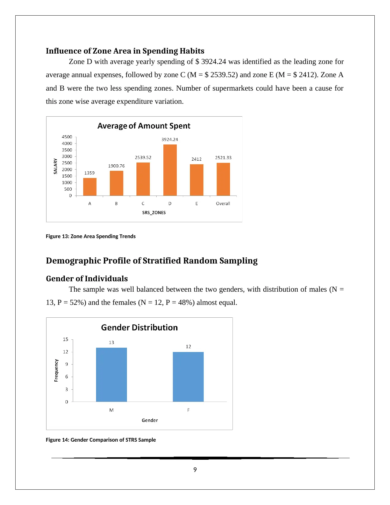
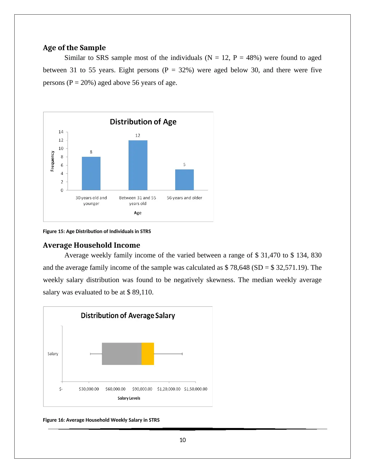
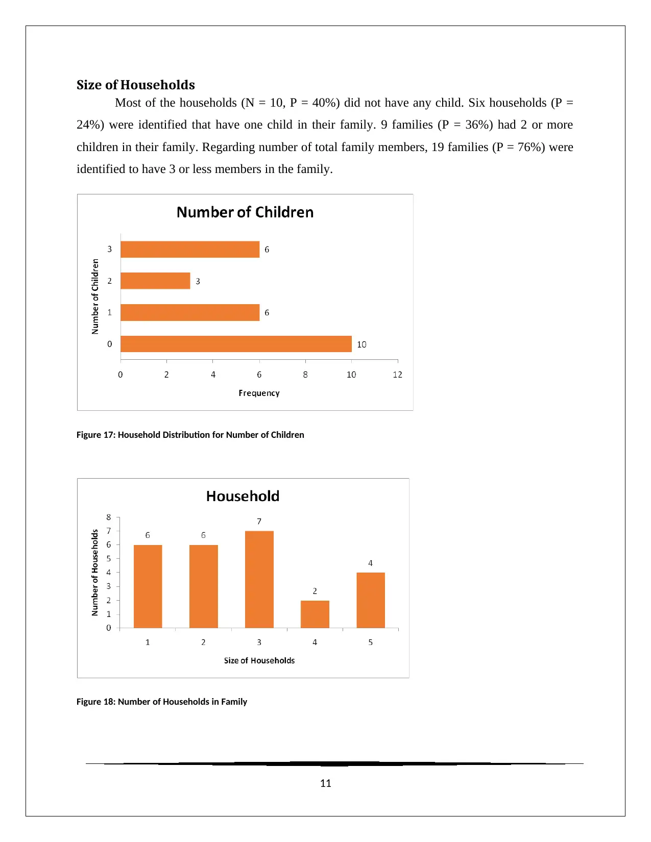
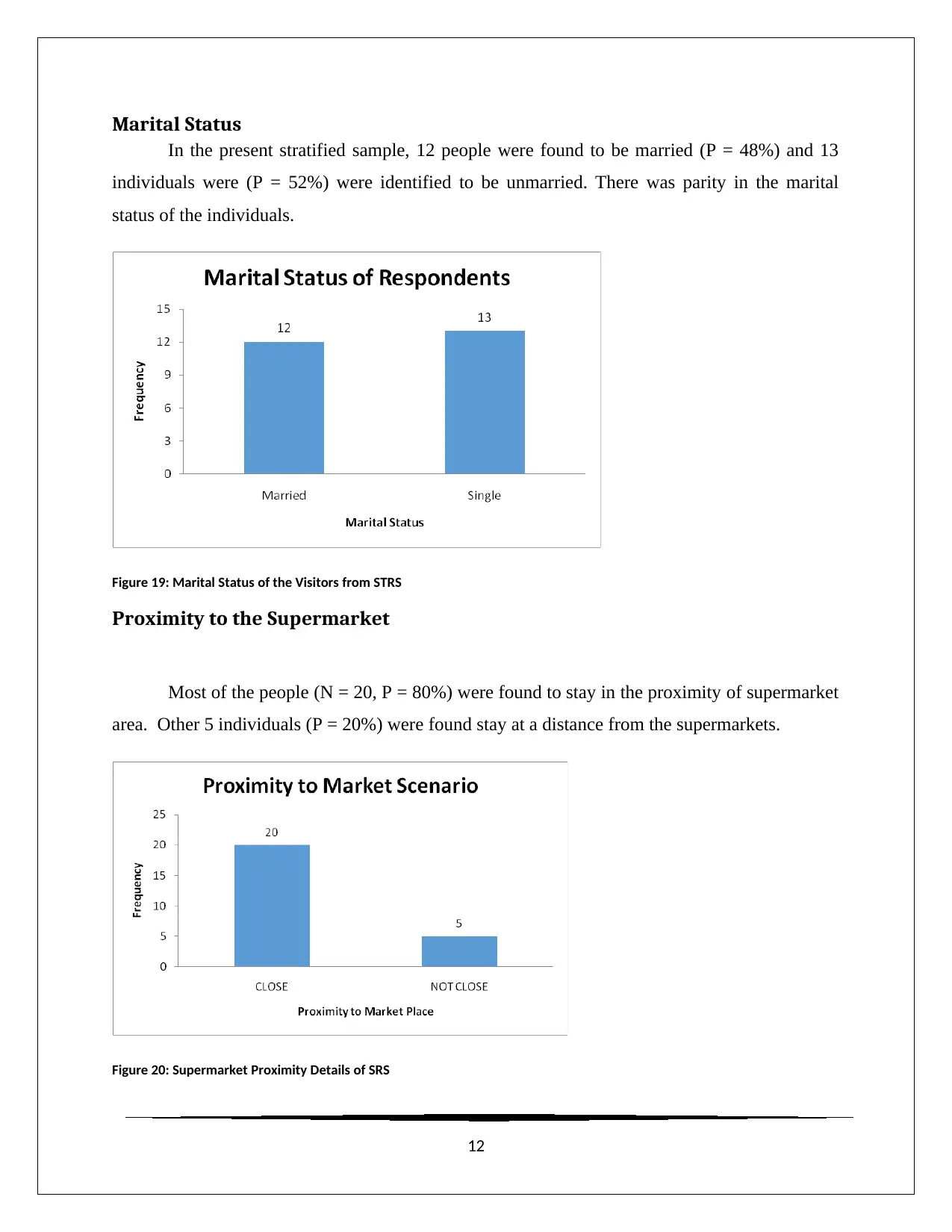
This report analyzes the relationship between individuals' yearly expenses and their supermarket purchases, categorized by zone. Two samples, one using Simple Random Sampling (SRS) and the other using Stratified Random Sampling (STRS), were collected from a population of 1000 individuals. The study examines demographic profiles, including gender, age, household income, and marital status, and their influence on spending habits. Key findings include the impact of zone area on spending, comparisons of male and female salaries, and an inferential analysis testing the supermarket chain's claim about the possibility of increased expenditure towards service improvement based on yearly average spending. The report provides detailed descriptive profiles of both the SRS and STRS samples, highlighting differences in average yearly purchases, debt levels, and proportion of debt to income, offering insights into consumer behavior and spending patterns.

Relation of Yearly Expenses with Supermarket
Purchases – A Zone Wise Inference
1

Introduction
The present article attempts to identify the description of the income and expenditure of
individuals. The research also undertook the effort to identify the relation between household
income levels and expenses made in supermarket purchase. The data was categorized on the
zone basis; and the influence of the yearly expenditure budget in supermarket purchases was also
investigated. The work moreover found the impact of the average yearly spending on increase of
spending to improve services in the supermarket (Hunneman, Verhoef, and Sloot, 2015).
Two samples of size 25 each were collected from a population of 1000 individuals. The
first sample was selected by Simple Random Sampling (SRS) and the second sample was
selected by Stratified Random Sampling (STRS) technique. For STRS, five observations were
randomly selected from each zone. The population was balanced between male (N = 484, P =
48.4%) and female (N = 516, P = 51.6%) individuals. The modal value of the age category of the
people was centered between 31 and 55 years of age. Zone C was identified as the region with
most number of individuals (N = 690, P = 69%), whereas zone E had least number of purchasers
(N = 33, P = 3.3%) of products from the supermarkets. Mean of average weekly salaries was
found to be $ 73,295.40 (SD = $ 23367.09), and the average yearly expenses was $ 2,387.72.
The SRS sample was obtained by assigning random numbers to each individual
observation, and the entire dataset was sorted in ascending order of random numbers. The first
25 sample were selected from the rearranged data set. The STRS sample was first sorted for
zones, and then for random numbers in ascending order. The 25 collected samples included first
5 samples from each zone arranged in ascending order. The stratified sample was expected to
contain less fluctuation for the continuous variables.
2

Descriptive Profile of Simple Random Sample
Gender of Individuals
The sample was well balanced between the two genders, with slight skewed towards the
males (N = 14, P = 56%) compared to that of the females (N = 11, P = 44%).
Figure 1: Gender Comparison of SRS Sample
Age of the Sample
Age categories of the individuals were provided instead of exact age, and most of the
individuals (N = 12, P = 48%) were found to aged between 31 to 55 years. Eight persons (P =
32%) were aged below 30, and there were five persons (P = 20%) aged above 56 years of age.
Hence, the sample seemed to be normally distributed with respected to the age of the individuals.
Figure 2: Age Distribution of Individuals in SRS
3

Average Household Income
Average weekly family income of the varied between a range of $ 35,060 to $ 109,290
and the average family income of the sample was calculated as $ 73,782 (SD = $ 20, 732.29).
The weekly salary distribution was found to be almost normally distributed with a slight negative
skewness. The median weekly average salary was evaluated to be at $ 87,970.
Figure 3: Average Household Weekly Salary
Size of Households
Most of the households (N = 11, P = 44%) did not have any child. nine households (P =
36%) were identified that have one child in their family. Only 5 families (P = 20%) had 2 or
more children in their family. Regarding number of total family members, 9 families (P = 36%)
were identified to have 3 members in the family. There were 12 households (P = 48%) which had
2 or less members in their family.
Figure 4: Household Distribution for Number of Children
4

Figure 5: Number of Households in Family
Marital Status
In the present sample, 13 people were found to be married (P = 52%) and 12 individuals
were (P = 48%) were identified to be unmarried. There was no disproportion in the marital status
of the individuals.
Figure 6: Marital Status of the Visitors
Proximity to the Supermarket
Most of the people (N = 15, P = 60%) were found to stay in the proximity of supermarket
area. Other 10 individuals (P = 40%) were found stay at a distance from the supermarkets.
Proximity to market areas is supposed to be an influencing factor for additional amount of
individual spending.
5

Figure 7: Supermarket Proximity Details of SRS
Zone of the Households
In the current sample, predominant presence of people from zone C was noted (N = 18, P
= 72%). Among the five zones, presence from zone A and E was minor (N = 1, P = 4%),
followed by presence from zone D (N= 2, P = 8%) and zone B (N = 3, P = 12%). The inferential
results could be influenced by the predominant presence of people from zone C in the sample.
Figure 8: Zone Distribution of Sample
6

Yearly Purchases
Average yearly purchase of the sample was $ 2521.33 (SD = $ 908.47), where the
minimum average yearly expenditure was $ 1359 and the maximum average yearly spending
was $ 4856.16. The sampling distribution for average yearly purchase was found to be positively
skewed (S = 1.09), and the median yearly expenditure was at $ 2397.26.
Figure 9: Box Plot for Yearly Expenses
Debt Levels
Average amount of non mortgage debt of the sample was $ 7451.78 (SD = $ 31176.01),
where the minimum average expenditure for consumption goods or services was $ 22,810 and
the maximum average expenditure for consumption goods or services was as high as $ 147,980.
The sampling distribution for average yearly purchase was found to be normally distributed, and
the median expenditure was at $ 90,030.
Figure 10: Box Plot of Average Non Mortgage Expenses
7

Proportion of Debt to Income Level
People were found to spend 11.2% of their weekly income on an average. The maximum
spending was found to be 26.9% of their weekly salary. The distribution for non mortgage debt
for the sample was almost normally distributed (S = 0.82), and the median of the debt ratio was
found to be at 9.67%.
Figure 11: Expenditure Proportion Box Plot
Comparison of Salary of Males and Females
Males were observed to be better paid than females. Average salary of males (M = $
77,487.14) was found to be higher than that of the females (M = $ 69,068.18). The median of
weekly average salary was also greater for males (ME = $ 80,045) compare to that of the females
(ME = $ 75,040).
Figure 12: Side by side Box Plot for Average Salary
8

Influence of Zone Area in Spending Habits
Zone D with average yearly spending of $ 3924.24 was identified as the leading zone for
average annual expenses, followed by zone C (M = $ 2539.52) and zone E (M = $ 2412). Zone A
and B were the two less spending zones. Number of supermarkets could have been a cause for
this zone wise average expenditure variation.
Figure 13: Zone Area Spending Trends
Demographic Profile of Stratified Random Sampling
Gender of Individuals
The sample was well balanced between the two genders, with distribution of males (N =
13, P = 52%) and the females (N = 12, P = 48%) almost equal.
Figure 14: Gender Comparison of STRS Sample
9

Age of the Sample
Similar to SRS sample most of the individuals (N = 12, P = 48%) were found to aged
between 31 to 55 years. Eight persons (P = 32%) were aged below 30, and there were five
persons (P = 20%) aged above 56 years of age.
Figure 15: Age Distribution of Individuals in STRS
Average Household Income
Average weekly family income of the varied between a range of $ 31,470 to $ 134, 830
and the average family income of the sample was calculated as $ 78,648 (SD = $ 32,571.19). The
weekly salary distribution was found to be negatively skewness. The median weekly average
salary was evaluated to be at $ 89,110.
Figure 16: Average Household Weekly Salary in STRS
10

Size of Households
Most of the households (N = 10, P = 40%) did not have any child. Six households (P =
24%) were identified that have one child in their family. 9 families (P = 36%) had 2 or more
children in their family. Regarding number of total family members, 19 families (P = 76%) were
identified to have 3 or less members in the family.
Figure 17: Household Distribution for Number of Children
Figure 18: Number of Households in Family
11

Marital Status
In the present stratified sample, 12 people were found to be married (P = 48%) and 13
individuals were (P = 52%) were identified to be unmarried. There was parity in the marital
status of the individuals.
Figure 19: Marital Status of the Visitors from STRS
Proximity to the Supermarket
Most of the people (N = 20, P = 80%) were found to stay in the proximity of supermarket
area. Other 5 individuals (P = 20%) were found stay at a distance from the supermarkets.
Figure 20: Supermarket Proximity Details of SRS
12