MENG 438 Engineering Analysis: Logistic Model and ODE Solutions

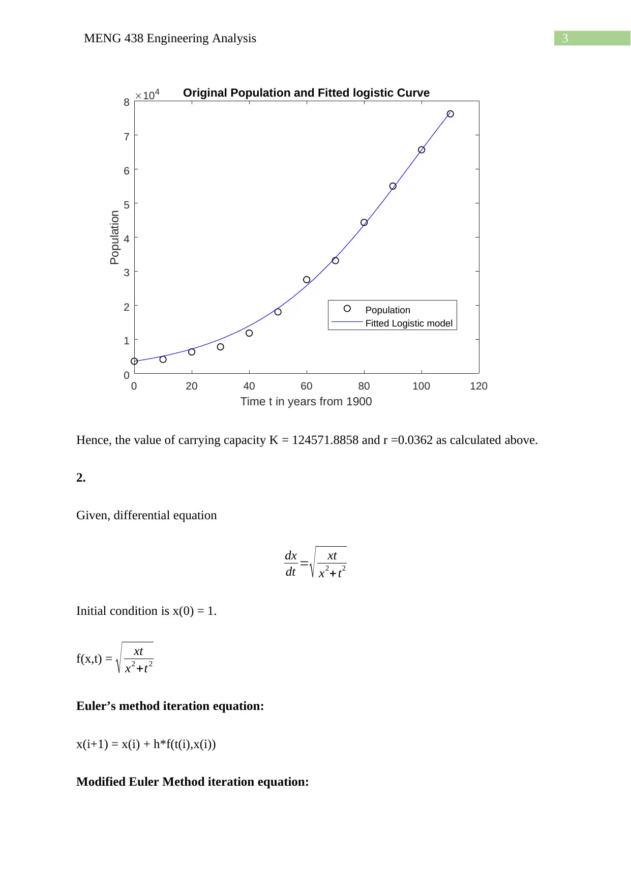
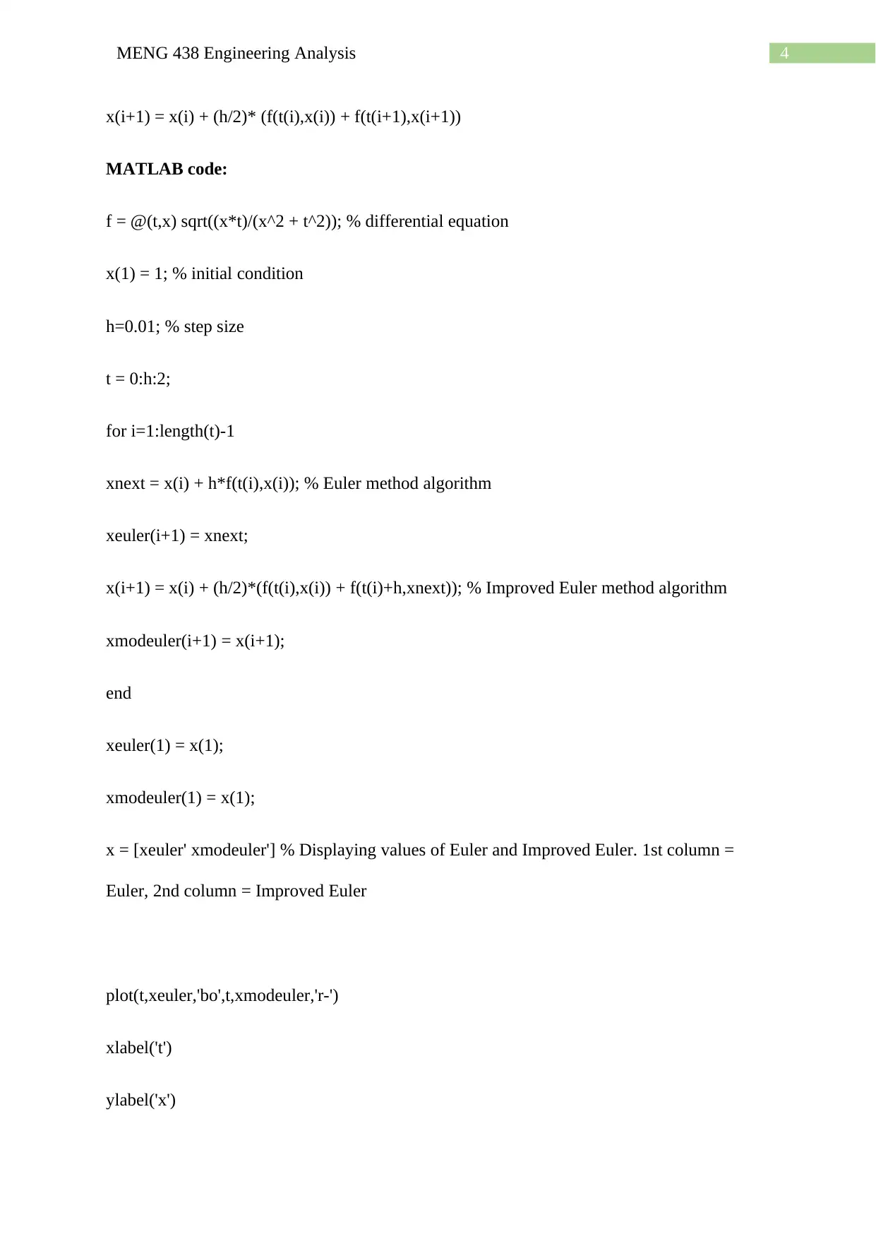
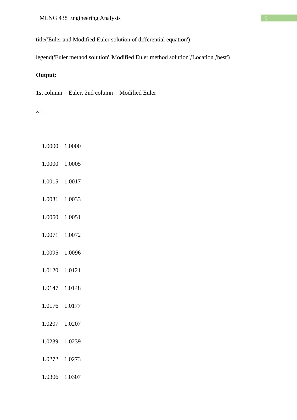
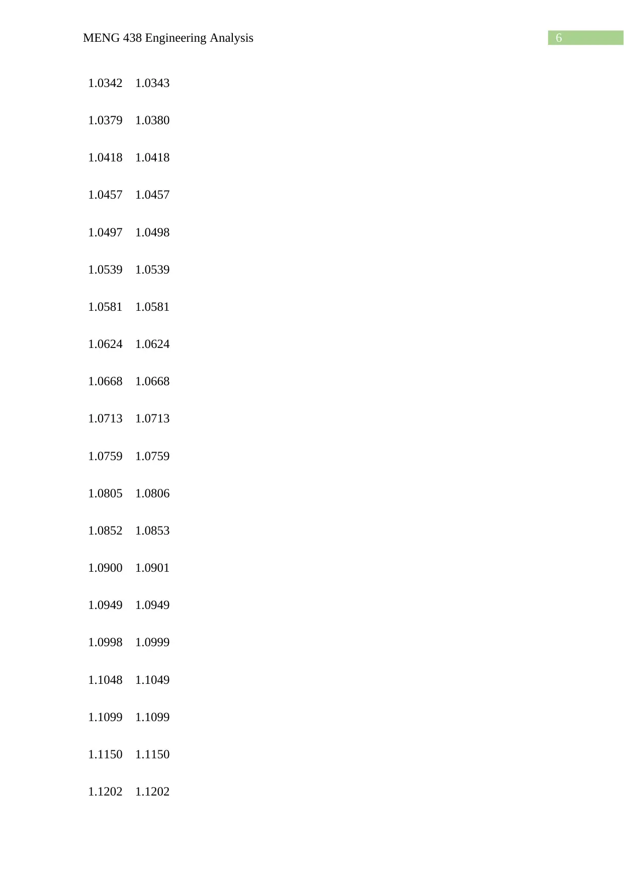
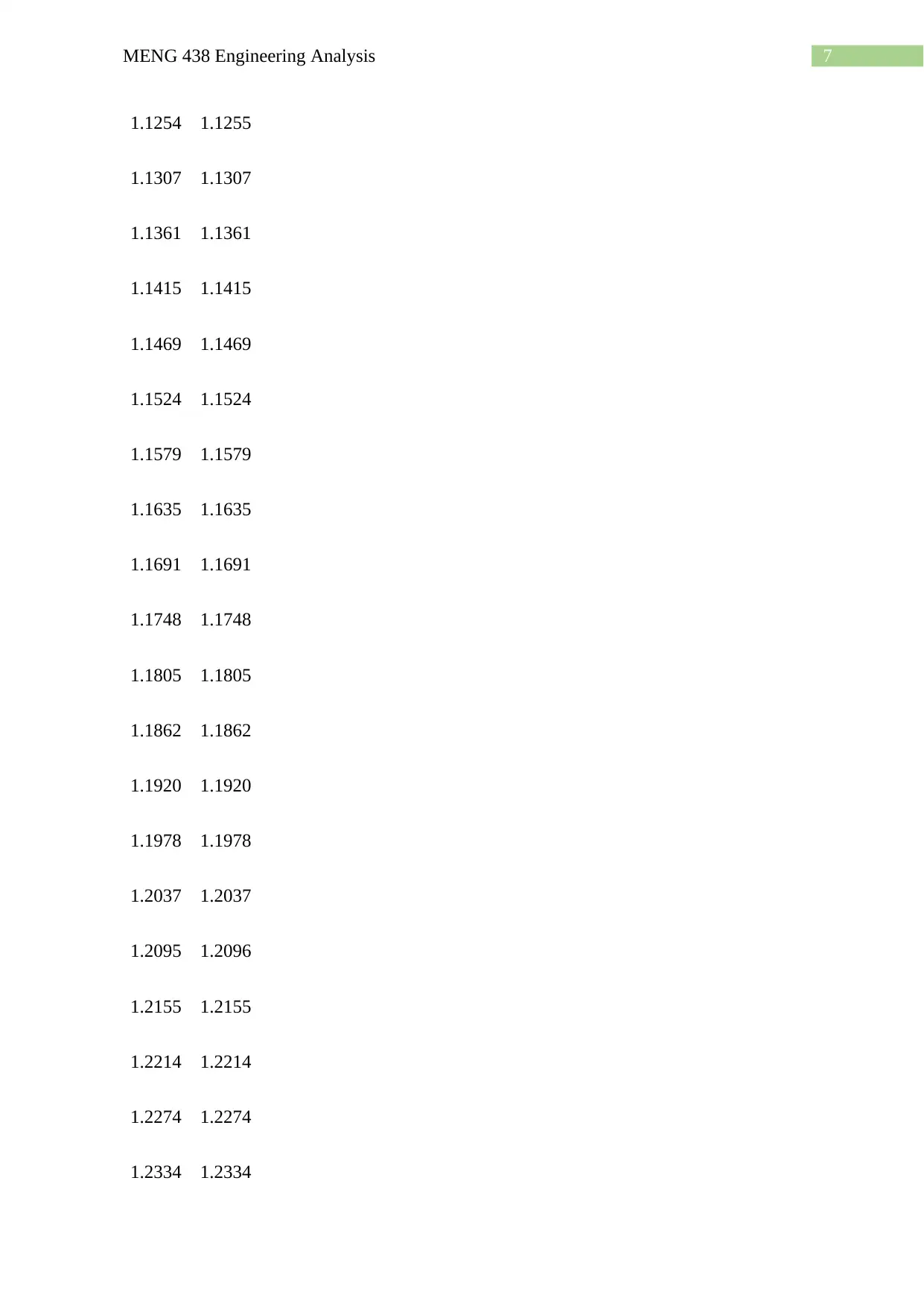
This document presents a comprehensive solution to a Mechanical Engineering assignment (MENG 438) focusing on engineering analysis. The assignment explores two main problems: the first involves fitting a logistic model to Bryan population data from 1900 to 2010 using MATLAB, determining the carrying capacity (K) and growth parameter (r) that minimizes the sum of square error. The second problem entails solving a given ordinary differential equation (ODE) using both Euler's method and the Modified Euler method implemented in MATLAB, with the results compared and plotted. Additionally, the ODE is solved using Simulink, demonstrating a different approach to the problem. The document includes detailed MATLAB code, outputs, and graphical representations of the solutions, providing a thorough analysis of the concepts and methods used.

Running head: MENG 438 Engineering Analysis
MENG 438 Engineering Analysis
Name of the Student
Name of the University
Author Note

1MENG 438 Engineering Analysis
1.
The regression equation of the logistic model is given by,
N(t) = N 0∗K
N 0+ ( K−N 0 ) ∗e−rt
N0 = Initial population = population at year 1900 = 3589
K = carrying capacity, r = growth parameter.
The logistic model is fitted to Bryan population data from 1900 to 2010 in 10 years interval.
The value of K and r of the best fitted model that is the model with minimum sum of square
error are calculated in MATLAB and then fitted as given below. The change in the objective
function or the logistic equation is below the default value of function tolerance which is
10^(-6) as given in MATLAB.
MATLAB code:
t = 0:10:110; % time t in years from 1900
p = [3589,4132,6307,7814,11842,18072,27542,33141,44337,55002,65660,76201]; %
population of Bryan
N0 = 3589; % specifying initial population N0
fun = @(param,t) (N0*param(1))./((N0 + (param(1) - N0).*exp(-param(2).*t))); % specifying
logistic model
param0 = [1,1]; % initial K and r values are assumed to be 1
lb = [0.01,0.01]; % specifying lower bound for K and r. K>0 and r>0
param_val = lsqcurvefit(fun,param0,t,p,lb,[]); % fitting non-linear logistic model

2MENG 438 Engineering Analysis
sprintf('The values of K = %.4f and r =%.4f which satisfies the least square
fit',param_val(1),param_val(2))
time = linspace(t(1),t(end));
plot(t,p,'ko',time,fun(param_val,time),'b-')
legend('Population','Fitted Logistic model','Location','best')
title('Original Population and Fitted logistic Curve')
xlabel('Time t in years from 1900')
ylabel('Population')
Output:
leastsqrfit
Local minimum possible.
lsqcurvefit stopped because the final change in the sum of squares relative to
its initial value is less than the default value of the function tolerance.
<stopping criteria details>
ans =
'The values of K = 124571.8858 and r =0.0362 which satisfies the least square fit'

3MENG 438 Engineering Analysis
0 20 40 60 80 100 120
Time t in years from 1900
0
1
2
3
4
5
6
7
8
Population
104 Original Population and Fitted logistic Curve
Population
Fitted Logistic model
Hence, the value of carrying capacity K = 124571.8858 and r =0.0362 as calculated above.
2.
Given, differential equation
dx
dt = √ xt
x2+ t2
Initial condition is x(0) = 1.
f(x,t) = √ xt
x2 +t2
Euler’s method iteration equation:
x(i+1) = x(i) + h*f(t(i),x(i))
Modified Euler Method iteration equation:

4MENG 438 Engineering Analysis
x(i+1) = x(i) + (h/2)* (f(t(i),x(i)) + f(t(i+1),x(i+1))
MATLAB code:
f = @(t,x) sqrt((x*t)/(x^2 + t^2)); % differential equation
x(1) = 1; % initial condition
h=0.01; % step size
t = 0:h:2;
for i=1:length(t)-1
xnext = x(i) + h*f(t(i),x(i)); % Euler method algorithm
xeuler(i+1) = xnext;
x(i+1) = x(i) + (h/2)*(f(t(i),x(i)) + f(t(i)+h,xnext)); % Improved Euler method algorithm
xmodeuler(i+1) = x(i+1);
end
xeuler(1) = x(1);
xmodeuler(1) = x(1);
x = [xeuler' xmodeuler'] % Displaying values of Euler and Improved Euler. 1st column =
Euler, 2nd column = Improved Euler
plot(t,xeuler,'bo',t,xmodeuler,'r-')
xlabel('t')
ylabel('x')

5MENG 438 Engineering Analysis
title('Euler and Modified Euler solution of differential equation')
legend('Euler method solution','Modified Euler method solution','Location','best')
Output:
1st column = Euler, 2nd column = Modified Euler
x =
1.0000 1.0000
1.0000 1.0005
1.0015 1.0017
1.0031 1.0033
1.0050 1.0051
1.0071 1.0072
1.0095 1.0096
1.0120 1.0121
1.0147 1.0148
1.0176 1.0177
1.0207 1.0207
1.0239 1.0239
1.0272 1.0273
1.0306 1.0307

6MENG 438 Engineering Analysis
1.0342 1.0343
1.0379 1.0380
1.0418 1.0418
1.0457 1.0457
1.0497 1.0498
1.0539 1.0539
1.0581 1.0581
1.0624 1.0624
1.0668 1.0668
1.0713 1.0713
1.0759 1.0759
1.0805 1.0806
1.0852 1.0853
1.0900 1.0901
1.0949 1.0949
1.0998 1.0999
1.1048 1.1049
1.1099 1.1099
1.1150 1.1150
1.1202 1.1202

7MENG 438 Engineering Analysis
1.1254 1.1255
1.1307 1.1307
1.1361 1.1361
1.1415 1.1415
1.1469 1.1469
1.1524 1.1524
1.1579 1.1579
1.1635 1.1635
1.1691 1.1691
1.1748 1.1748
1.1805 1.1805
1.1862 1.1862
1.1920 1.1920
1.1978 1.1978
1.2037 1.2037
1.2095 1.2096
1.2155 1.2155
1.2214 1.2214
1.2274 1.2274
1.2334 1.2334

8MENG 438 Engineering Analysis
1.2394 1.2394
1.2455 1.2455
1.2516 1.2516
1.2577 1.2577
1.2639 1.2639
1.2700 1.2700
1.2762 1.2762
1.2824 1.2824
1.2887 1.2887
1.2949 1.2949
1.3012 1.3012
1.3075 1.3075
1.3138 1.3139
1.3202 1.3202
1.3266 1.3266
1.3329 1.3329
1.3393 1.3393
1.3457 1.3458
1.3522 1.3522
1.3586 1.3586

9MENG 438 Engineering Analysis
1.3651 1.3651
1.3716 1.3716
1.3781 1.3781
1.3846 1.3846
1.3911 1.3911
1.3976 1.3976
1.4042 1.4042
1.4108 1.4108
1.4173 1.4173
1.4239 1.4239
1.4305 1.4305
1.4371 1.4371
1.4438 1.4438
1.4504 1.4504
1.4571 1.4571
1.4637 1.4637
1.4704 1.4704
1.4771 1.4771
1.4837 1.4837
1.4904 1.4904

10MENG 438 Engineering Analysis
1.4971 1.4972
1.5039 1.5039
1.5106 1.5106
1.5173 1.5173
1.5241 1.5241
1.5308 1.5308
1.5376 1.5376
1.5443 1.5443
1.5511 1.5511
1.5579 1.5579
1.5647 1.5647
1.5715 1.5715
1.5783 1.5783
1.5851 1.5851
1.5919 1.5919
1.5987 1.5987
1.6055 1.6055
1.6124 1.6124
1.6192 1.6192
1.6260 1.6260

11MENG 438 Engineering Analysis
1.6329 1.6329
1.6397 1.6397
1.6466 1.6466
1.6535 1.6535
1.6603 1.6603
1.6672 1.6672
1.6741 1.6741
1.6810 1.6810
1.6879 1.6879
1.6947 1.6947
1.7016 1.7016
1.7085 1.7085
1.7155 1.7155
1.7224 1.7224
1.7293 1.7293
1.7362 1.7362
1.7431 1.7431
1.7500 1.7500
1.7570 1.7570
1.7639 1.7639