Homogeneity Analysis of Rainfall Time Series for Australian Stations

This report presents a comprehensive analysis of rainfall data collected from numerous meteorological stations across Australia, spanning from 1978 to 2015. The primary objective is to assess the homogeneity of the climate data, employing tools such as the MASH method, Pettitt Test, Buishand Test, and Double Mass Curve Tests. The study examines various parameters, including temperature, precipitation levels, and precipitation duration, to identify breakpoints and trends. The findings reveal that most breakpoints in the temperature data occurred after the year 2000, likely due to the replacement of older meteorological instruments with modern equipment. The analysis indicates a decreasing trend in precipitation and an increasing trend in temperatures across Australia during the study period. Corrections applied using the MASH method led to reductions in annual precipitation, maximum temperature, minimum temperature, and average temperature. The report also discusses the influence of station location and data collection methods on the accuracy of the results. The research contributes to a better understanding of climate variability and provides valuable insights into the reliability of long-term climate records.

Meteorological Stations in Australia selected for
the Homogeneity Analysis of Rainfall Time
series.

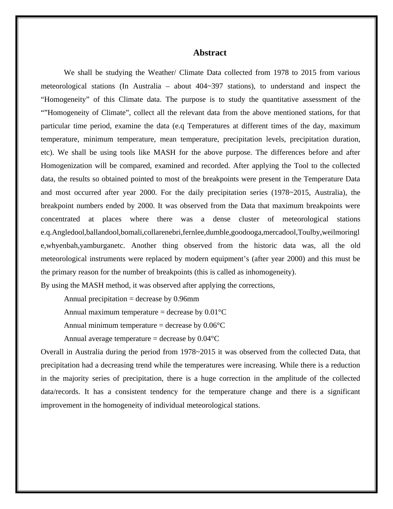
Abstract
We shall be studying the Weather/ Climate Data collected from 1978 to 2015 from various
meteorological stations (In Australia – about 404~397 stations), to understand and inspect the
“Homogeneity” of this Climate data. The purpose is to study the quantitative assessment of the
“”Homogeneity of Climate”, collect all the relevant data from the above mentioned stations, for that
particular time period, examine the data (e.q Temperatures at different times of the day, maximum
temperature, minimum temperature, mean temperature, precipitation levels, precipitation duration,
etc). We shall be using tools like MASH for the above purpose. The differences before and after
Homogenization will be compared, examined and recorded. After applying the Tool to the collected
data, the results so obtained pointed to most of the breakpoints were present in the Temperature Data
and most occurred after year 2000. For the daily precipitation series (1978~2015, Australia), the
breakpoint numbers ended by 2000. It was observed from the Data that maximum breakpoints were
concentrated at places where there was a dense cluster of meteorological stations
e.q.Angledool,ballandool,bomali,collarenebri,fernlee,dumble,goodooga,mercadool,Toulby,weilmoringl
e,whyenbah,yamburganetc. Another thing observed from the historic data was, all the old
meteorological instruments were replaced by modern equipment’s (after year 2000) and this must be
the primary reason for the number of breakpoints (this is called as inhomogeneity).
By using the MASH method, it was observed after applying the corrections,
Annual precipitation = decrease by 0.96mm
Annual maximum temperature = decrease by 0.01°C
Annual minimum temperature = decrease by 0.06°C
Annual average temperature = decrease by 0.04°C
Overall in Australia during the period from 1978~2015 it was observed from the collected Data, that
precipitation had a decreasing trend while the temperatures were increasing. While there is a reduction
in the majority series of precipitation, there is a huge correction in the amplitude of the collected
data/records. It has a consistent tendency for the temperature change and there is a significant
improvement in the homogeneity of individual meteorological stations.

Contents
Abstract..................................................................................................................................................................2
Objective................................................................................................................................................................4
Introduction...........................................................................................................................................................5
Description.............................................................................................................................................................7
Literature Review...................................................................................................................................................8
Research problem and scope...............................................................................................................................23
Resources Required..............................................................................................................................................24
Stakeholder/ Industry and their Plausible benefit................................................................................................25
Constraints...........................................................................................................................................................26
Conclusion............................................................................................................................................................27
References............................................................................................................................................................28

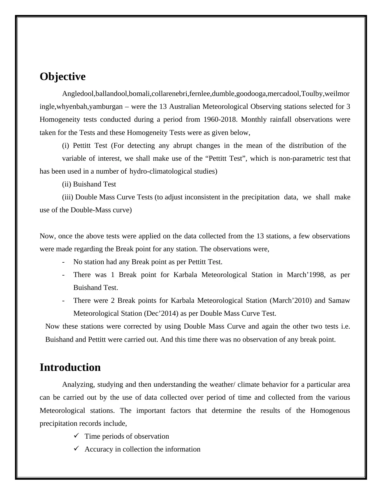
Objective
Angledool,ballandool,bomali,collarenebri,fernlee,dumble,goodooga,mercadool,Toulby,weilmor
ingle,whyenbah,yamburgan – were the 13 Australian Meteorological Observing stations selected for 3
Homogeneity tests conducted during a period from 1960-2018. Monthly rainfall observations were
taken for the Tests and these Homogeneity Tests were as given below,
(i) Pettitt Test (For detecting any abrupt changes in the mean of the distribution of the
variable of interest, we shall make use of the “Pettitt Test”, which is non-parametric test that
has been used in a number of hydro-climatological studies)
(ii) Buishand Test
(iii) Double Mass Curve Tests (to adjust inconsistent in the precipitation data, we shall make
use of the Double-Mass curve)
Now, once the above tests were applied on the data collected from the 13 stations, a few observations
were made regarding the Break point for any station. The observations were,
- No station had any Break point as per Pettitt Test.
- There was 1 Break point for Karbala Meteorological Station in March’1998, as per
Buishand Test.
- There were 2 Break points for Karbala Meteorological Station (March’2010) and Samaw
Meteorological Station (Dec’2014) as per Double Mass Curve Test.
Now these stations were corrected by using Double Mass Curve and again the other two tests i.e.
Buishand and Pettitt were carried out. And this time there was no observation of any break point.
Introduction
Analyzing, studying and then understanding the weather/ climate behavior for a particular area
can be carried out by the use of data collected over period of time and collected from the various
Meteorological stations. The important factors that determine the results of the Homogenous
precipitation records include,
 Time periods of observation
 Accuracy in collection the information

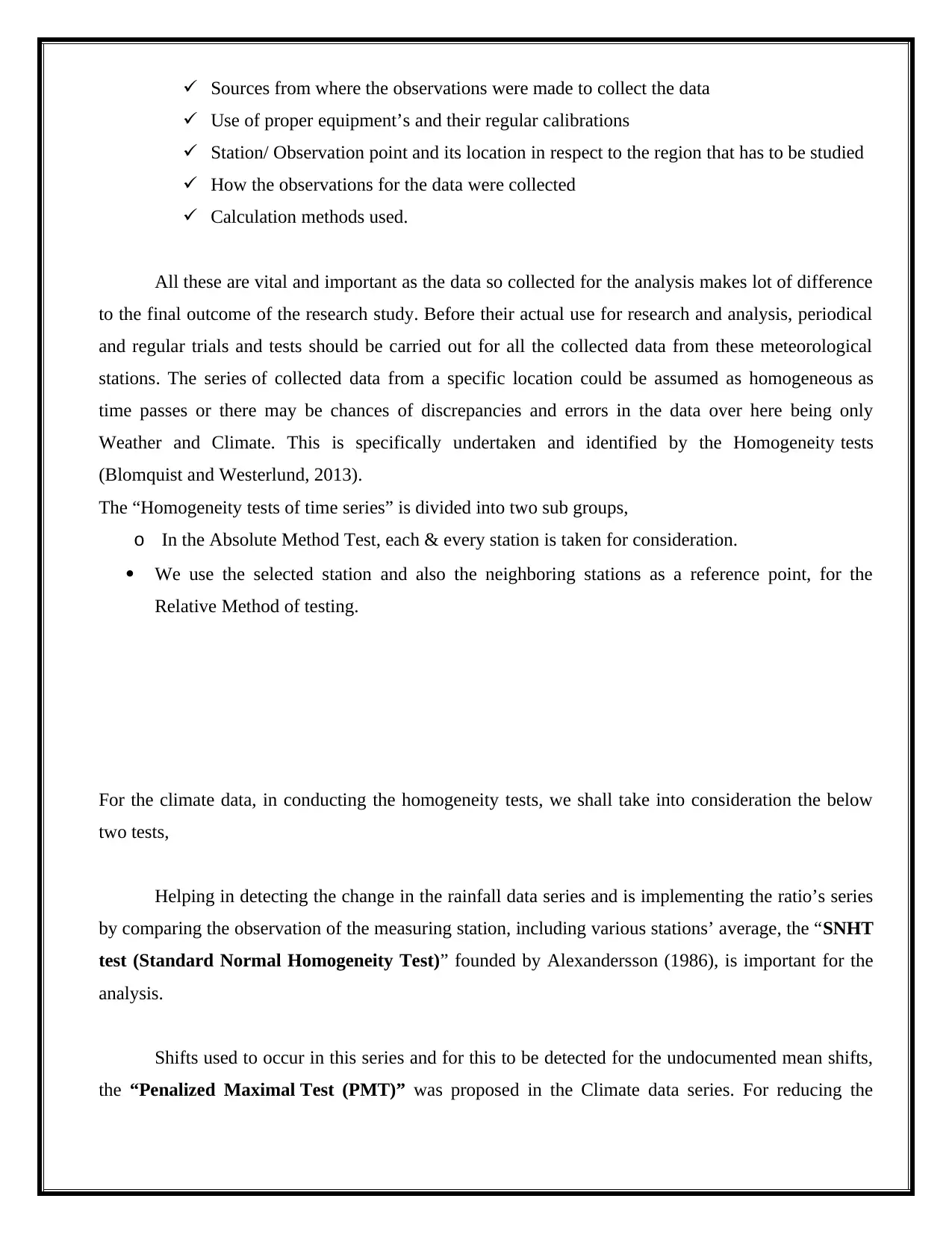
 Sources from where the observations were made to collect the data
 Use of proper equipment’s and their regular calibrations
 Station/ Observation point and its location in respect to the region that has to be studied
 How the observations for the data were collected
 Calculation methods used.
All these are vital and important as the data so collected for the analysis makes lot of difference
to the final outcome of the research study. Before their actual use for research and analysis, periodical
and regular trials and tests should be carried out for all the collected data from these meteorological
stations. The series of collected data from a specific location could be assumed as homogeneous as
time passes or there may be chances of discrepancies and errors in the data over here being only
Weather and Climate. This is specifically undertaken and identified by the Homogeneity tests
(Blomquist and Westerlund, 2013).
The “Homogeneity tests of time series” is divided into two sub groups,
o In the Absolute Method Test, each & every station is taken for consideration.
 We use the selected station and also the neighboring stations as a reference point, for the
Relative Method of testing.
For the climate data, in conducting the homogeneity tests, we shall take into consideration the below
two tests,
Helping in detecting the change in the rainfall data series and is implementing the ratio’s series
by comparing the observation of the measuring station, including various stations’ average, the “SNHT
test (Standard Normal Homogeneity Test)” founded by Alexandersson (1986), is important for the
analysis.
Shifts used to occur in this series and for this to be detected for the undocumented mean shifts,
the “Penalized Maximal Test (PMT)” was proposed in the Climate data series. For reducing the

uneven sample sizes’ effect on the detection power, PMT makes sure that each candidate’s relative
position in the change point into the account.
Kept for observation at a single systematic change for an independent time series in Europe, the above
two methodologies were implemented for analysing the data. Failing to identify the change points near
the end of the observing series, PMT was more accurate to locate all the change points in a series (Deo,
2010).
Now to overcome this hurdle, they proposed the use of another tool called the SUR model of
testing (SUR model could be seen either as the general linear model’s simplification, where specific
coefficients are restricted in the matrix must be zero or according to the general linear model on right
hand side the parameters are permitted to be distinct in every equation)
Various observers were testing different methods and tests on homogeneity data to get the best
results. The four tests, Von Neumann Ratio (VNR) Test, Pettitt Test, MASH Test and the Buishand
Range (BR)Test, were used for the European climate data. While in Ethiopia, Seleshiand Camberlin
was using the MASH technique for multiple analyses for a series (Gijbels and Omelka, 2012).
Now, the results from these tests and analysis were divided into three groups based upon their
reliability and worthiness. They were divided as Suspect, Doubtful, and Useful based on the times the
tests were rejecting the Null Hypothesis.
(“Null Hypothesis” refers to a basic statement or a default position where there contains no
relationship among a couple of measured phenomena or contains no link between the groups).
Now the parameters used during the observation and testing were based on annual values both
for temperatures and precipitation. The annual mean of daily absolute differences, including the diurnal
temperature range, were the variables used for the observations for the testing in case of “Temperature”
parameter.
Total wet days (limit parameter 1mm) in a year were taken as the value for the precipitation.
In 3 places namely, Northern Africa, , Gonzalez-Rouco in Iberian Peninsula and Southern France in the
year 2001, SNHT test models were used, analyzed and examined for the homogeneity of precipitation.
While in Czech Republic, Stepanek made the use of Bivariate Test, SNHT, and Easterling/ Peterson
Test for detection of homogeneities in air temperature and precipitation data (Kaspar, Hannak and
Schreiber, 2016).

As in the previous observation and analysis in Australia, 36 meteorological stations were
chosen for this project’s study for assessing the homogeneity of rainfall (annual) as per the method of
Wijngaard et al.
Adapting different tools like Normal Ration method, all the numbers and data was completed in
the missing rainfall record. Out of the two test methods, Absolute was chosen because of the random
rainfall patterns and also the random geographical distribution of observation stations. For tests which
include a hydrologic design and study, homogenous rainfall is preferred. This was the reason that
Relative Test was not used as the stations which were selected for the investigation had a very less
positive correlation among them. The Rain which refers to a tool that is used for collection of
precipitation data is not uniformly taken. There are discrepancies in the position, exposure time, height
used, type of gauge used for the data collection etc. All the above factors make it difficult to gauge the
accuracy of the data collected from these stations. Hence there is always a doubt factor in the data
collected as these will influence the data so collected (Etuk and Mohamed, 2014).
Now to overcome this uncertainty and to have a better insight of the record, a popular tool is
used for plotting all the data collected from on station to the data collected from another station. This
tool is called as the “Double Mass Curve”. For the purpose of Analysis “Double Mass Analysis
Curve” is considered to be an important tool in checking the consistency of a hydrological or
meteorological record. This method depends on a hypothesis where every single item of the data
recorded from the population is said to be consistent (Kocsis and Anda, 2018).
This same test was used on the three data’s collected and they observed that there was not much change
and effect on the data. Therefore they came to the conclusion that no correction will be applied. The
data had not much deviation and hence no correction. Pettitt Test, Double Mass Curve Tests and
Buishand Test were used in the homogeneity test for the Australian observation stations.
Description
Various locations are characterized based on specific climate conditions as per their latitude as
Australia is a vast continent. Most part this nation gets sunshine that is greater than 3,000 hours each
year, but overall Australia is actually temperate climate. Christmas is celebrated in the mid-summer

and etc, as Australia is in the southern hemisphere. June to August is the winter season (where average
temperature is 13° Celsius) while the Summer starts in the month of December till March where the
average temperature is 29° Celsius. The winters are rainy and very cool, yet it offers a lot of daylight.
The summer is sweltering with mild nights. Most of travelers travel in the Eastern part of Australia, and
like the temperature out there. Typically hot when moving through north and cold in the south, coastal
area’s ocean soften weather condition in general in Australia.(Lavanya, Radha and Arulanandu, 2018).
With average rainfall at 216mm, ranging from 100~1200, Monsoon is generally from December to
February. Nora Head, Walpole, Moree, Watsonia, C0bar, whyenbah (1960-2018) and Hilla Station are
the Meteorological observation stations in Australia that we will consider for our project.
Literature Review
For Australia, a research on the extended historical high quality rainfall data set was carried
out by this paper (Lavery, Joung and Nicholls, 2019). Coupled with statistical tests, after an exhaustive
search of documentation on the Australian rainfall sites, this paper was able to identify the 191 high
quality long term rainfall records. By enhancing the spatial convergence for the feasible to perform on
an area for the average of the precipitation for Australia, it can reliable monitor the rainfall treads for
the most of Australia. Related to all the long term rainfall stations which are still operating, it involves
the comprehensive searching of the relevant documents and papers. To check for the possible
homogeneities in the data, statistical tests were also employed in the selection process. The point of
measurement for precipitation will be the main objective of this project and for this confidentially
constructing by using the identified reliable rainfall records will be employed. It is suitable for various
climatologically and hydrological studies as it contains spatial and temporal distribution. To perform
the real average of precipitation across Australia, enhanced spatial coverage is more appropriate.
Represented by the climates of that station, we shall use the Thiessen Polygon method which consists
of the defined areas around each of this station. The “Emrpicail rule” will be used for calculations and
for that we shall require a minimum number of stations for a reasonably safe estimate. 329
representation sites in Australia will be considered for this Rule and they are involved in areal rainfall
estimates, which again are based on strongly of the variability of the rainfall over the domain. For
different types of climatic and hydrological studies, the data set described here provides the adequate
spatial and temporal distribution. To estimate the curve model, we shall be using the double mass curve
test as presented (Dourado et al., 2010). To obtain accurate value of energy, crack equivalent concept is
utilized. It also provides consistent values for data reduction schemes, determines the energy of this

wood species and proposes the methodologies for the performance. For analysing the data for rainfall
during 1968 to 2018 and for calculating the significance value, we shall use the double mass curve test.
This method does not require monitoring the data as this method migrates the influence of the
scatter of wood elastic properties on the measure energy. Including the linear and nonlinear modeling
for analysis, the statically and graphical technique’s (Test conflict using creftest, 2012) are included
here. The Pettit test, double mass curve test and Buishand test are the tests included in this study of the
homogeneity test. For calculating the “p” value and the correlation, we shall apply the double curve test
for the selected Australia stations, which is from the year 1960 to 2018 rainfall data for the two
stations. In the Pettit test and the Double Mass curve tests, after conducting the 2 tests, it was found
that there was no break point for any station, but for the Buishand test there was a break point in certain
stations. For finding the correlation coefficient of rainfall data, we shall use the double mass curve test.
By using the Double mass curve test as mentioned in this paper (Pirnia et al., 2018), we shall be
analyzing the Rainfall data. The double mass curve test shall be applied on chosen stations are Fitzroy
and Brisbane and the time series for the rainfall variables will be from 1960 to 2018. From 1960 to
2018, the rainfall changes on the stations had significant respective decreasing and increasing trends at
the 0.01 confidence level, as per the results of the tests. The rainfall decrease and increase was as the
climate variability contributed 57.76% and 42.25% respectively to it. The stream flow regimes can
change significantly as the factor of hydrological cycle for climate change and temperature are altered.
Using the double mass curve test we shall calculate the average rainfall and the Rainfall values
during 960 to 2018 decreased. Compare the rainfall values from 2000 to 2018 and the climate changes
in 1960 to 2000. The significance level is 0.96 and confidence level is 0.01 for the rainfall results
during the period. Analysing the correlation for the rainfall values during 1960 to 2018, was carried out
by the double mass curve test. Any change in rainfall data, which was divided into two periods for
calculations, compares the two periods of the data for the tests and this was indicated by the
Correlation analysis. We shall carry out the testing of the null hypothesis value and also same time we
shall calculate the value of “p”. Now we have the following conditions,
data is considered to be significant if, p < 0.05
data is considered to be not significant if, p>= 0.05
We shall calculate the double mass cure test and also the significant level for both periods.
Analysis of the correlation for the data and the explanation of the double mass cure test, will be carried
out in this paper. The seasonal precipitation maxima shall follow with time the varying parameters and
this is assumed this paper (Hanel and Buishand, 2010). Also we shall calculate the coefficient for

rainfall data during 1960-2018 by using the location parameter which varies with these regions.
Between the scale and location parameter, we shall calculate the ratio parameter. The shape parameter
will remain the same for the rainfall data which has been used for the comparison of the two periods
and for a predefined region. The location parameter for RCM simulations in winter will be used as the
number of RCM simulations conducted is the dispersion coefficient. Based on low number of stations,
the gridding will be the observations used. For the analysis of the extreme value which is the selection
of the threshold we shall have the approach (Roth, Jongbloed and Buishand, 2015). This method for
analysing the data has been used in many environment applications. The graphical tools represented by
the mean excess will be the threshold selection and regionalized versions of the threshold stability.
Based on the bootstrap distribution, now we shall introduce the spatially averaged Buishand test statics.
Compared to the method which does not take into account the regional information, the proposed
regional method leads to an increased sensitivity for too low thresholds. An application to rainfall data
from the stations will be presented using simulated data.
Exceeding the sample size as per this paper (Gijbels and Omelka, 2012), the number of
variables used in the method. Cannot carry out the calculation on the matrix of the pairwise differences
and data analysts as, they are based on the basis of parametric assumptions. A matrix of pairwise is
used in this paper based on test of homogeneity and design of the anova. Calculating to obtain the test
statistic, the approach was based on the means of within group distance. Calculates from the rainfall
data given and collected, it is used for the hypothesis test for random variable. The Test statistic is used
to calculate the value of “p” and also the null hypothesis is rejected or not depends upon these criteria.
The measurement of the degree of agreement between two comparable data is taken and calculations
carried out for determining this null hypothesis and under this sampling distribution of the test statistic
is carried out. This is called as Null distribution. To find out the values of probability on this data and
the value of “p”, we shall make use of the above data.
The significance of the data depends upon the relation of “p” with 0.05. i.e.
Data is significant if p < 0.05
Data is not significant if p >= 0.05
The significant value is based on the Test statistic, which is also used for calculating the value of “p”
It was found that cloned code is more stable by comparing the stability of cloned code nod for
analysing the data (Harder and Göde, 2012).Calculating the correlation and significant value, R
language is used for analysing the data. Finer grained measurement was used in the research and also
this will require frequently voiced assumptions and less maintenance efforts. Able to manage the

memory hierarchies, used and managed explicitly in software’s exposed to the programmer, as
mentioned in this research paper (Jang et al., 2012). With embedded systems, these same hierarchies are
used vastly in the multicore architectures. This application uses Code memory, which is found on higher
level memory. As a requirement for this application, the specialized linker is the one who manually
generates the overlay structure. The statistical analysis is computed for the given sets where the worst
case number of conflict misses between two different code segments exists. For the rainfall data during
1960 to 2018, we shall use for analyzing the statically data, the R code. For the rainfall data between
two stations, we have calculated the correlation and significant value. Not considering the program
context, we shall propose a new and alternative, automatic code overlay generate technique in this
paper.
For analysing the data, we shall use the R Code in this research paper (Ledford, 2010), where
the R code will be widely used for the encoding by using the statically analysis. We shall discuss and
explain the procedure for analysing the data using the R code. Provided for various operating systems,
this language is used for data mining. It is the command line interface for analysing the data
statistically, the significant level, the “p” value and finally to calculate the correlation coefficient.
It displays the time series for each data and at the same time makes use of the graphical
technique for statically analysis. We have calculated the time series during 1960 to 2018 for the rainfall
data for the meteorological stations in Australia. For the modeling in the RNA landscape, we have used
the computational methods. For the detecting the small regulatory targets in RNA and for predicting
the RNA structures we shall make use of this data. Comprehensively compiled in to catalogues, the
RNA molecules are found in various environmental conditions and in different tissues. How a certain
type of gene would be expressed in a particular tissue and predicting its form, are some of the uses of
this RNA structures. We have also discovered by using this method that human genome in 95% of
humans is alternatively spliced.
.
THEORY
1.1 Pettit Test
The Pettit test indicates a non-parametric test which is utilized in various
hydro climatological studies for detecting a variable interest and the abrupt changes
in its mean distribution. This “Petit Test” allows and identifies in an unclear point in
time, a single move, with the help of the rank-based test, which is derived from the

3
Mann-Whitney two-sample test. As there are no distributional presumptions, this
above test can be used often for distinguishing the shifts in the boundaries(Kumbuyo
et al., 2014).
At a continuous data for detecting the break point [10]:
Observations (X) are ranked ranging between 1 to N (that is X1, X2, …,XN
Estimate the value of Vi,N:
Vi=N + 1 — 2Rii = 1, 2, 3, …, N …………….………….……...….
(1) where Riis the rank of Xi in a sample of “N” observations.
1. Estimating the U value:
U i= U i–1 + Vi ……………………………………………… …….. (2)
U 1= V 1………….……………………………………......……..….. (3)
2. Detecting the value of KN:
KN = max1ŠiŠN |Ui| ……...…………………...……......………...... (4)
3. Estimate the
value of POÆ: 6.
POÆ = 2
e
6K2
{– N
}
(N +N)
………………….……………........…..……… (5)
If POÆ € α, where α denotes the test’ statistical significance, and does not consider the null hypothesis.
Buishand Test
Buishand Test is carried out for observation of the mean and the cumulative
deviation of it and how this affects and the mean value. It is based on the mean and its
cumulative deviation and the adjusted sums.
From Buishand [1] null hypothesis which makes an observation that there is a
normal distribution of data, it is homogenous and the alternative hypothesis indicates that