Comprehensive Report on Micro and Macro Economics Principles
VerifiedAdded on 2022/12/14
|16
|4105
|346
Report
AI Summary
This report provides a detailed analysis of key concepts in microeconomics and macroeconomics. Section A explores the budget constraint, illustrating consumer behavior and its graphical representation. Section B delves into microeconomic principles, including the calculation of profit-maximizing quantity and price under perfect competition, the behavior of firms, and the conditions for long-run economic profit. Section C shifts to macroeconomics, explaining the real exchange rate and its significance. The report uses examples and equations to clarify the concepts, providing a comprehensive overview of economic principles. The report also includes an analysis of market models, assumptions underlying perfect competition, and the impact of factors like identical goods and ease of entry and exit on market dynamics. The report concludes with discussion of real exchange rates and their implications.
Principles of Economics
1
1
Paraphrase This Document
Need a fresh take? Get an instant paraphrase of this document with our AI Paraphraser
Contents
Section A – Microeconomics...........................................................................................................3
A1. Budget constraint.............................................................................................................3
Section B – Microeconomics...........................................................................................................6
Question B1............................................................................................................................6
Section C – Macroeconomics........................................................................................................11
C1 Real Exchange Rate (RER).............................................................................................11
Section D – Macroeconomics........................................................................................................12
Question D3..........................................................................................................................12
References......................................................................................................................................16
2
Section A – Microeconomics
A1. Budget constraint
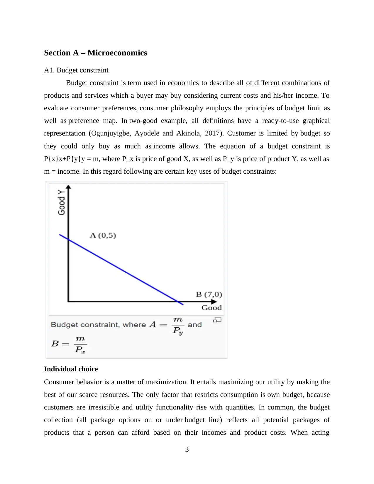
Budget constraint is term used in economics to describe all of different combinations of
products and services which a buyer may buy considering current costs and his/her income. To
evaluate consumer preferences, consumer philosophy employs the principles of budget limit as
well as preference map. In two-good example, all definitions have a ready-to-use graphical
representation (Ogunjuyigbe, Ayodele and Akinola, 2017). Customer is limited by budget so
they could only buy as much as income allows. The equation of a budget constraint is
P{x}x+P{y}y = m, where P_x is price of good X, as well as P_y is price of product Y, as well as
m = income. In this regard following are certain key uses of budget constraints:
Individual choice
Consumer behavior is a matter of maximization. It entails maximizing our utility by making the
best of our scarce resources. The only factor that restricts consumption is own budget, because
customers are irresistible and utility functionality rise with quantities. In common, the budget
collection (all package options on or under budget line) reflects all potential packages of
products that a person can afford based on their incomes and product costs. When acting
3
A1. Budget constraint
Budget constraint is term used in economics to describe all of different combinations of
products and services which a buyer may buy considering current costs and his/her income. To
evaluate consumer preferences, consumer philosophy employs the principles of budget limit as
well as preference map. In two-good example, all definitions have a ready-to-use graphical
representation (Ogunjuyigbe, Ayodele and Akinola, 2017). Customer is limited by budget so
they could only buy as much as income allows. The equation of a budget constraint is
P{x}x+P{y}y = m, where P_x is price of good X, as well as P_y is price of product Y, as well as
m = income. In this regard following are certain key uses of budget constraints:
Individual choice
Consumer behavior is a matter of maximization. It entails maximizing our utility by making the
best of our scarce resources. The only factor that restricts consumption is own budget, because
customers are irresistible and utility functionality rise with quantities. In common, the budget
collection (all package options on or under budget line) reflects all potential packages of
products that a person can afford based on their incomes and product costs. When acting
3
⊘ This is a preview!⊘
Do you want full access?
Subscribe today to unlock all pages.
Trusted by 1+ million students worldwide
rationally, a buyer should opt to buy products at the level on preference map where most
preferred accessible indifference curve becomes tangent to budget constraint. Tangent point (xy
coordinate) reflects the number of products x as well as y that a buyer can buy to get most out
of budget. It's worth noting that the best consumption package isn't necessarily an interior option.
When optimality condition's response corresponds to an unfeasible package, the consumer's best
option would be corner solution, implying that the products or inputs perfect replacements. The
expansion direction is line that connects all levels of tangency between indifference curve as well
as budget constraint.
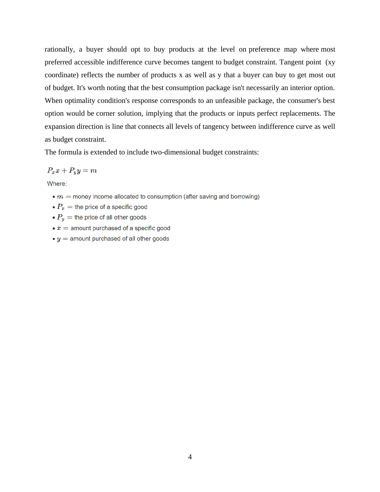
The formula is extended to include two-dimensional budget constraints:
4
preferred accessible indifference curve becomes tangent to budget constraint. Tangent point (xy
coordinate) reflects the number of products x as well as y that a buyer can buy to get most out
of budget. It's worth noting that the best consumption package isn't necessarily an interior option.
When optimality condition's response corresponds to an unfeasible package, the consumer's best
option would be corner solution, implying that the products or inputs perfect replacements. The
expansion direction is line that connects all levels of tangency between indifference curve as well
as budget constraint.
The formula is extended to include two-dimensional budget constraints:
4
Paraphrase This Document
Need a fresh take? Get an instant paraphrase of this document with our AI Paraphraser
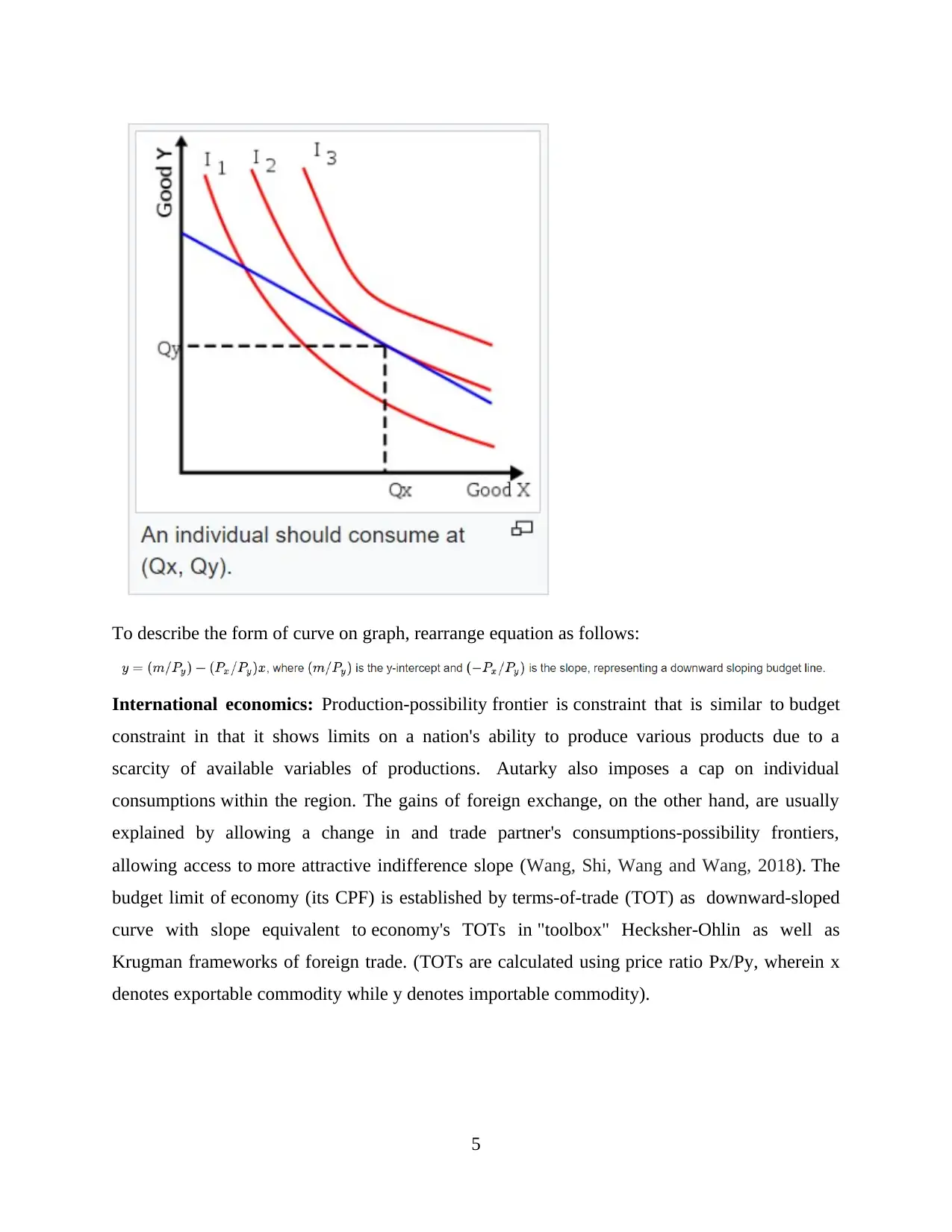
To describe the form of curve on graph, rearrange equation as follows:
International economics: Production-possibility frontier is constraint that is similar to budget
constraint in that it shows limits on a nation's ability to produce various products due to a
scarcity of available variables of productions. Autarky also imposes a cap on individual
consumptions within the region. The gains of foreign exchange, on the other hand, are usually
explained by allowing a change in and trade partner's consumptions-possibility frontiers,
allowing access to more attractive indifference slope (Wang, Shi, Wang and Wang, 2018). The
budget limit of economy (its CPF) is established by terms-of-trade (TOT) as downward-sloped
curve with slope equivalent to economy's TOTs in "toolbox" Hecksher-Ohlin as well as
Krugman frameworks of foreign trade. (TOTs are calculated using price ratio Px/Py, wherein x
denotes exportable commodity while y denotes importable commodity).
5
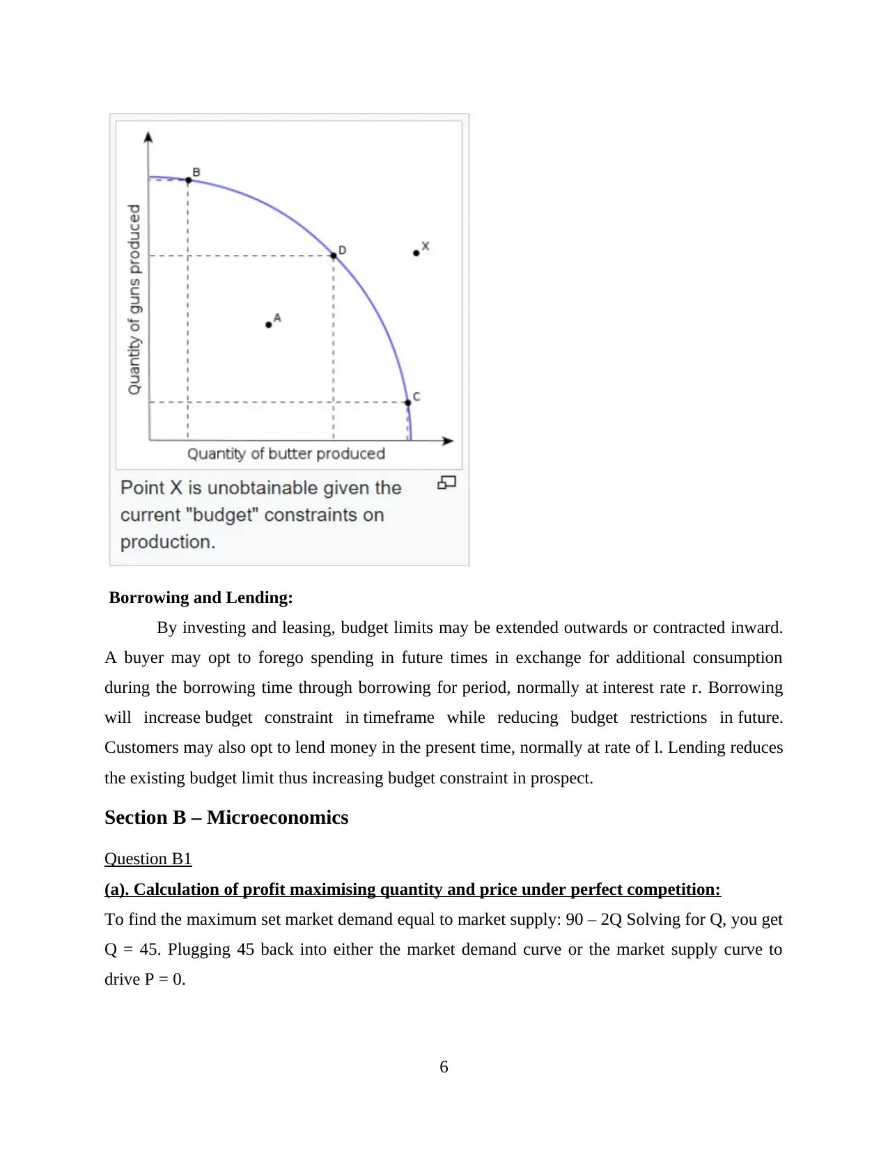
Borrowing and Lending:
By investing and leasing, budget limits may be extended outwards or contracted inward.
A buyer may opt to forego spending in future times in exchange for additional consumption
during the borrowing time through borrowing for period, normally at interest rate r. Borrowing
will increase budget constraint in timeframe while reducing budget restrictions in future.
Customers may also opt to lend money in the present time, normally at rate of l. Lending reduces
the existing budget limit thus increasing budget constraint in prospect.
Section B – Microeconomics
Question B1
(a). Calculation of profit maximising quantity and price under perfect competition:
To find the maximum set market demand equal to market supply: 90 – 2Q Solving for Q, you get
Q = 45. Plugging 45 back into either the market demand curve or the market supply curve to
drive P = 0.
6
⊘ This is a preview!⊘
Do you want full access?
Subscribe today to unlock all pages.
Trusted by 1+ million students worldwide
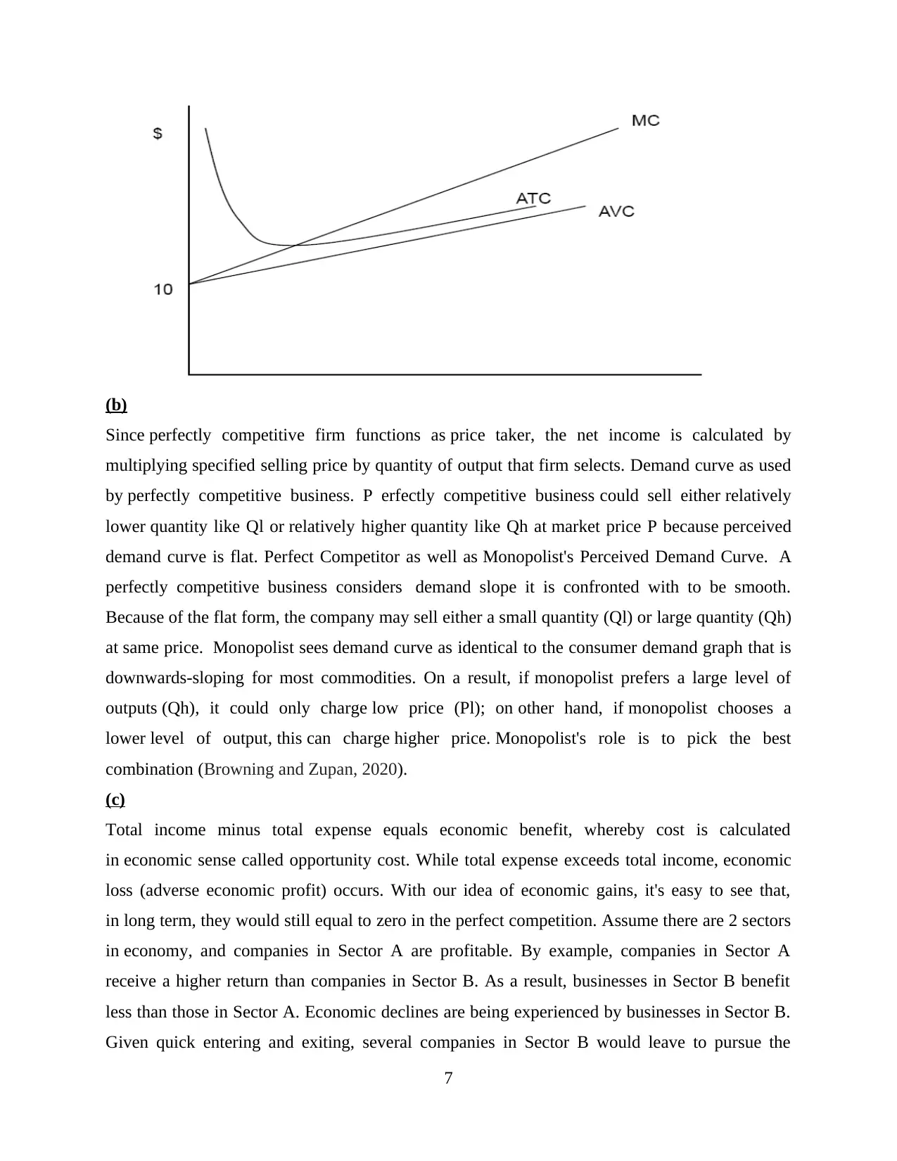
(b)
Since perfectly competitive firm functions as price taker, the net income is calculated by
multiplying specified selling price by quantity of output that firm selects. Demand curve as used
by perfectly competitive business. P erfectly competitive business could sell either relatively
lower quantity like Ql or relatively higher quantity like Qh at market price P because perceived
demand curve is flat. Perfect Competitor as well as Monopolist's Perceived Demand Curve. A
perfectly competitive business considers demand slope it is confronted with to be smooth.
Because of the flat form, the company may sell either a small quantity (Ql) or large quantity (Qh)
at same price. Monopolist sees demand curve as identical to the consumer demand graph that is
downwards-sloping for most commodities. On a result, if monopolist prefers a large level of
outputs (Qh), it could only charge low price (Pl); on other hand, if monopolist chooses a
lower level of output, this can charge higher price. Monopolist's role is to pick the best
combination (Browning and Zupan, 2020).
(c)
Total income minus total expense equals economic benefit, whereby cost is calculated
in economic sense called opportunity cost. While total expense exceeds total income, economic
loss (adverse economic profit) occurs. With our idea of economic gains, it's easy to see that,
in long term, they would still equal to zero in the perfect competition. Assume there are 2 sectors
in economy, and companies in Sector A are profitable. By example, companies in Sector A
receive a higher return than companies in Sector B. As a result, businesses in Sector B benefit
less than those in Sector A. Economic declines are being experienced by businesses in Sector B.
Given quick entering and exiting, several companies in Sector B would leave to pursue the
7
Paraphrase This Document
Need a fresh take? Get an instant paraphrase of this document with our AI Paraphraser
higher profits achievable in Sector A. Here, supply curve in Sector B would move to left as a
result, increasing costs and earnings. Supply curve in Sector A would turn to right as former
Sector B companies join Sector A, lowering income in A. The trend of companies exiting
Industry B or entering Sector A will proceed until all sectors are profitable at zero. That implies a
significant long-run outcome: in system with perfectly open economies, economic income would
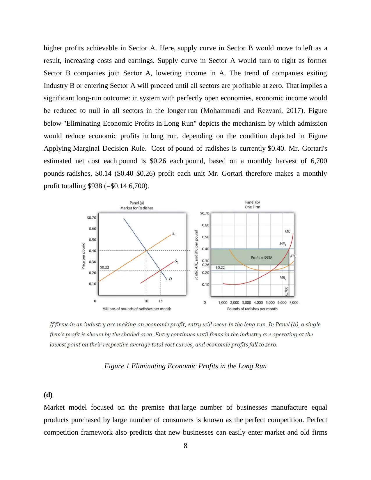
be reduced to null in all sectors in the longer run (Mohammadi and Rezvani, 2017). Figure
below "Eliminating Economic Profits in Long Run" depicts the mechanism by which admission
would reduce economic profits in long run, depending on the condition depicted in Figure
Applying Marginal Decision Rule. Cost of pound of radishes is currently $0.40. Mr. Gortari's
estimated net cost each pound is $0.26 each pound, based on a monthly harvest of 6,700
pounds radishes. $0.14 ($0.40 $0.26) profit each unit Mr. Gortari therefore makes a monthly
profit totalling $938 (=$0.14 6,700).
Figure 1 Eliminating Economic Profits in the Long Run
(d)
Market model focused on the premise that large number of businesses manufacture equal
products purchased by large number of consumers is known as the perfect competition. Perfect
competition framework also predicts that new businesses can easily enter market and old firms
8
result, increasing costs and earnings. Supply curve in Sector A would turn to right as former
Sector B companies join Sector A, lowering income in A. The trend of companies exiting
Industry B or entering Sector A will proceed until all sectors are profitable at zero. That implies a
significant long-run outcome: in system with perfectly open economies, economic income would
be reduced to null in all sectors in the longer run (Mohammadi and Rezvani, 2017). Figure
below "Eliminating Economic Profits in Long Run" depicts the mechanism by which admission
would reduce economic profits in long run, depending on the condition depicted in Figure
Applying Marginal Decision Rule. Cost of pound of radishes is currently $0.40. Mr. Gortari's
estimated net cost each pound is $0.26 each pound, based on a monthly harvest of 6,700
pounds radishes. $0.14 ($0.40 $0.26) profit each unit Mr. Gortari therefore makes a monthly
profit totalling $938 (=$0.14 6,700).
Figure 1 Eliminating Economic Profits in the Long Run
(d)
Market model focused on the premise that large number of businesses manufacture equal
products purchased by large number of consumers is known as the perfect competition. Perfect
competition framework also predicts that new businesses can easily enter market and old firms
8
can easily exit. Finally, it is assumed that both buyers as well as sellers possess full knowledge of
market trends (Yi-ran, 2018). In this regard following some key assumptions underlying
perfectly competitive model hold in UK potatoes market, as follows:
Identical Goods
In such perfectly competitive market for potatoes, one unit of potatoes cannot be distinguished
from the others on any grounds. In potatoes market, goods are identical and all sellers sell
potatoes.
A Large Number of Buyers and Sellers:
Since there're so many purchasers and sellers no-one will have an impact on the stock price,
irrespective as to how much they buying or selling. In perfectly competitive sector, a business
can respond to price changes, but it could not influence prices it spends for inputs or gets
for output.
Ease of Entry and Exit
The belief that other companies will find it easier to reach perfectly competitive market means
that there will be still more rivalry. Firms in market must contend with not only vast number of
competitors, but also prospect of other competitors entering the market. We'll look at how
convenience of entry relates to the long-term viability of economic income later. If entrance is
simple, new businesses can be attracted easily by the prospect of higher economic profits. This
won't if getting in is tough. The ideal competition model expects that both entry and exit are
easy. The presumption of a simple exit reinforces the assumption of a simple entrance. Assume a
company is contemplating entering a certain industry. It can be simple to get in, however
imagine how tough it is to get out. Providers of variables of output to industry companies, for
instance, may be willing to accept new businesses as long as they sign longer-term contracts.
Contracts like this could make exiting the market challenging and expensive. If this is the case, a
company will be reluctant to enter the market in first place. It is easier to enter if you have a
simple escape (Mohammadi and Rezvani, 2019).
Complete Information
One expects that all vendors have full knowledge of markets, technologies, as well as all details
related to market activity. There is no detail about manufacturing processes that a single seller
requires that isn't accessible to any those sellers. When one seller has a competitive advantage
over another, such as insider knowledge of a lower-cost processing process, seller could exercise
9
⊘ This is a preview!⊘
Do you want full access?
Subscribe today to unlock all pages.
Trusted by 1+ million students worldwide
some leverage over market pricing—the seller will no longer be price taker. The assumption of
information supply in the ideal competition model means that information could be accessed
at lower cost. Consumers and businesses are more likely to access information at reduced cost if
it is available. Whatever the source, believe that it is inexpensive enough for customers and
businesses to purchase and sell products and services at retail rates dictated by intersection of
demands and supply curves.
10
Paraphrase This Document
Need a fresh take? Get an instant paraphrase of this document with our AI Paraphraser
Section C – Macroeconomics
C1 Real Exchange Rate (RER)
Real exchange rate multiplied by price ratio between 2 countries, P/P*, yields real
exchange rate (RER) among two currencies. As a result, RER is eP*/P. Consider Germany's
relationship with United States. A increase in RER may be used to indicate appreciation (as IMF
can do) or decline (as IMF can do). It's all a matter of etiquette. Let's describe RER so that an
increase signifies an increase in the actual exchange price of Germany. In such example, e
is dollar-euro market price, P is average German value of products as well as P* is average US
price of products. A single symbolic product, such as Big Mac, McDonald's burger served in
several nations in almost equivalent varieties, can be used to calculate the real exchange
rates between 2 nations. If real exchange rates for such good is 1, burger in United States will
cost same as one in, perhaps, Germany when represented in common currency. If Big Mac
charges $5.30 in United States then €4.50 in Germany, this will be case. The buying power parity
of dollar and euro are same in such one-product environment (where values match exchanging
rates as well as RER is 1. But let's say the burger costs €5.40 in the Germany. Which means this
costs 20% more in eurozone than it does in United States, implying that euro is 20percent
overbought against dollar. Since same good could be bought more cheaper in one nation than
in other, there must be stress on nominal exchange rate level to move if the actual exchange rate
level becomes that overvalued. Even so, purchasing dollars, using them to purchase Big Macs
in United States for around 1 euro, as well as then selling them in the Germany for 1.2 euros will
make economic perception. Arbitrage is the practice of profiting from pricing differences. When
arbitrageurs acquire dollars to acquire Big Macs to offer in the Germany, demand towards
dollars increases, as does nominal exchange rate, until price in both countries is same—the RER
corresponds to 1 (Calderón and Kubota, 2018). Most costs, like logistics, trade restrictions and
consumer tastes, obstruct a straightforward market analysis in real world. The basic idea is that
as RERs deviate, currencies are under pressure to adjust. Overvalued currencies are under stress
to depreciate, while undervalued currencies are under stress to appreciation. It may get more
difficult if considerations like government policy obstruct natural exchange price equilibration,
which is a common source of trade conflicts. In the case of Big Mac, average price in
the Germany (across all McDonald's restaurants) is around €4.50, while average price in United
11
States is around $5.30. (as-of July 2017). Taking 1.18-dollar exchange level for Big Mac in
the Germany. The RER becomes 1.18 x 4.5/5.3, or 1.18. As a result, the euro does not appear to
be underrated or overvalued in relation to dollar at current exchange rate (Guzman, Ocampo and
Stiglitz, 2018).
Section D – Macroeconomics
Question D3
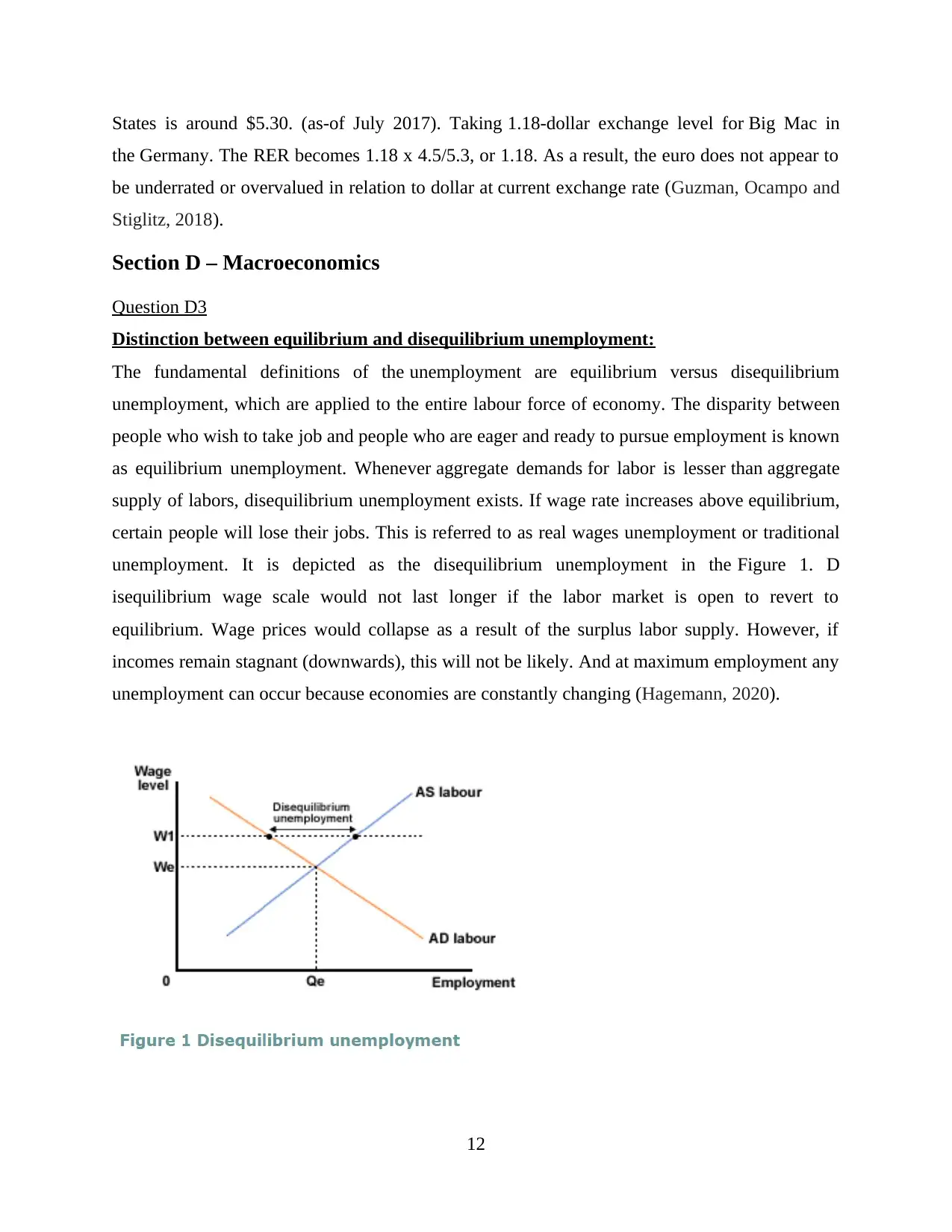
Distinction between equilibrium and disequilibrium unemployment:
The fundamental definitions of the unemployment are equilibrium versus disequilibrium
unemployment, which are applied to the entire labour force of economy. The disparity between
people who wish to take job and people who are eager and ready to pursue employment is known
as equilibrium unemployment. Whenever aggregate demands for labor is lesser than aggregate
supply of labors, disequilibrium unemployment exists. If wage rate increases above equilibrium,
certain people will lose their jobs. This is referred to as real wages unemployment or traditional
unemployment. It is depicted as the disequilibrium unemployment in the Figure 1. D
isequilibrium wage scale would not last longer if the labor market is open to revert to
equilibrium. Wage prices would collapse as a result of the surplus labor supply. However, if
incomes remain stagnant (downwards), this will not be likely. And at maximum employment any
unemployment can occur because economies are constantly changing (Hagemann, 2020).
12
the Germany. The RER becomes 1.18 x 4.5/5.3, or 1.18. As a result, the euro does not appear to
be underrated or overvalued in relation to dollar at current exchange rate (Guzman, Ocampo and
Stiglitz, 2018).
Section D – Macroeconomics
Question D3
Distinction between equilibrium and disequilibrium unemployment:
The fundamental definitions of the unemployment are equilibrium versus disequilibrium
unemployment, which are applied to the entire labour force of economy. The disparity between
people who wish to take job and people who are eager and ready to pursue employment is known
as equilibrium unemployment. Whenever aggregate demands for labor is lesser than aggregate
supply of labors, disequilibrium unemployment exists. If wage rate increases above equilibrium,
certain people will lose their jobs. This is referred to as real wages unemployment or traditional
unemployment. It is depicted as the disequilibrium unemployment in the Figure 1. D
isequilibrium wage scale would not last longer if the labor market is open to revert to
equilibrium. Wage prices would collapse as a result of the surplus labor supply. However, if
incomes remain stagnant (downwards), this will not be likely. And at maximum employment any
unemployment can occur because economies are constantly changing (Hagemann, 2020).
12
⊘ This is a preview!⊘
Do you want full access?
Subscribe today to unlock all pages.
Trusted by 1+ million students worldwide
1 out of 16


Your All-in-One AI-Powered Toolkit for Academic Success.
+13062052269
info@desklib.com
Available 24*7 on WhatsApp / Email
![[object Object]](/_next/static/media/star-bottom.7253800d.svg)
Unlock your academic potential
Copyright © 2020–2026 A2Z Services. All Rights Reserved. Developed and managed by ZUCOL.