Microeconomic Analysis Report: Applications in Business and Government
VerifiedAdded on 2019/11/14
|27
|4727
|272
Report
AI Summary
This report provides a detailed analysis of microeconomic principles, offering valuable insights into various concepts and their applications. It begins with an examination of business cycles, including recession and expansion phases, and explores the causes of economic fluctuations. The report then delves into demand elasticity, examining price, cross, and income elasticities, and uses case studies to illustrate these concepts. Further, it covers market structures, including duopolies and oligopolies, and discusses the impact of barriers to entry, consumer exploitation, and government intervention. The report also analyzes cost curves and game theory, including payoff matrices. The document incorporates diagrams and tables to illustrate key concepts and provides a comprehensive overview of microeconomic analysis, making it a useful resource for students and professionals alike. This report is contributed by a student to be published on the website Desklib. Desklib is a platform which provides all the necessary AI based study tools for students.
Micro Economic Analysis September 20
2017
Micro Economic Analysis is very useful in making decision. This paper
gives various examples of micro economic concepts used in business
and government. These tools are useful for managers as well as policy
makers.
2017
Micro Economic Analysis is very useful in making decision. This paper
gives various examples of micro economic concepts used in business
and government. These tools are useful for managers as well as policy
makers.
Paraphrase This Document
Need a fresh take? Get an instant paraphrase of this document with our AI Paraphraser
Micro Economic Analysis
Contents
Table of Figures..............................................................................................................................2
Part A Case study........................................................................................................................... 4
Case 1......................................................................................................................................... 4
a) Business Cycles................................................................................................................4
b) Causes of Recession........................................................................................................ 6
Case 2......................................................................................................................................... 8
Part B........................................................................................................................................... 11
1. U Shaped Cost Curves.......................................................................................................11
2. Elasticity of Demand......................................................................................................... 15
a) Price Elasticity of Demand..................................................................................................17
b.1) Cross Elasticity of Demand............................................................................................19
b.2) Income elasticity of demand.........................................................................................20
Part C........................................................................................................................................... 23
a) Barriers to Entry................................................................................................................23
b) Consumer Exploitation......................................................................................................23
c) Government Intervention.................................................................................................24
Table of Figures
Diagram 1 Business Cycles...........................................................................................................................6
Diagram 2 Demand Side Illustration of Recession and Expansion ..............................................................8
Diagram 3 Market Indifference Curve.........................................................................................................9
Diagram 4 Marginal Product of Labour.....................................................................................................12
Diagram 5 Several Short Run Average Total Cost Curves are possible in the Long Run 14
Diagram 6 Long Run Average Total Costs for Various Plant Sizes..............................................................15
Diagram 7 Price Elasticity of Demand........................................................................................................19
Diagram 8 : The Kinked Demand curve for Non Collusive Oligopoly.........................................................23
Diagram 9 Demand Curve in a Non Collusive Oligopoly............................................................................24
Diagram 10 Oligopoly and Joint Profit Maximization................................................................................26
2
Micro Economic Analysis
Table 1 Pay-off Matrix in case of games........................................................................................9
Table 2 An Illustration of Income Elasticity of Demand with examples.......................................19
3
Table 1 Pay-off Matrix in case of games........................................................................................9
Table 2 An Illustration of Income Elasticity of Demand with examples.......................................19
3
⊘ This is a preview!⊘
Do you want full access?
Subscribe today to unlock all pages.
Trusted by 1+ million students worldwide
Micro Economic Analysis
Part A Case study
Case 1
a) Business Cycles
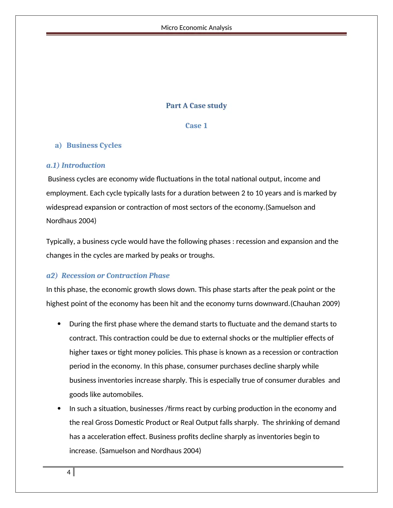
a.1) Introduction
Business cycles are economy wide fluctuations in the total national output, income and
employment. Each cycle typically lasts for a duration between 2 to 10 years and is marked by
widespread expansion or contraction of most sectors of the economy.(Samuelson and
Nordhaus 2004)
Typically, a business cycle would have the following phases : recession and expansion and the
changes in the cycles are marked by peaks or troughs.
a2) Recession or Contraction Phase
In this phase, the economic growth slows down. This phase starts after the peak point or the
highest point of the economy has been hit and the economy turns downward.(Chauhan 2009)
During the first phase where the demand starts to fluctuate and the demand starts to
contract. This contraction could be due to external shocks or the multiplier effects of
higher taxes or tight money policies. This phase is known as a recession or contraction
period in the economy. In this phase, consumer purchases decline sharply while
business inventories increase sharply. This is especially true of consumer durables and
goods like automobiles.
In such a situation, businesses /firms react by curbing production in the economy and
the real Gross Domestic Product or Real Output falls sharply. The shrinking of demand
has a acceleration effect. Business profits decline sharply as inventories begin to
increase. (Samuelson and Nordhaus 2004)
4
Part A Case study
Case 1
a) Business Cycles
a.1) Introduction
Business cycles are economy wide fluctuations in the total national output, income and
employment. Each cycle typically lasts for a duration between 2 to 10 years and is marked by
widespread expansion or contraction of most sectors of the economy.(Samuelson and
Nordhaus 2004)
Typically, a business cycle would have the following phases : recession and expansion and the
changes in the cycles are marked by peaks or troughs.
a2) Recession or Contraction Phase
In this phase, the economic growth slows down. This phase starts after the peak point or the
highest point of the economy has been hit and the economy turns downward.(Chauhan 2009)
During the first phase where the demand starts to fluctuate and the demand starts to
contract. This contraction could be due to external shocks or the multiplier effects of
higher taxes or tight money policies. This phase is known as a recession or contraction
period in the economy. In this phase, consumer purchases decline sharply while
business inventories increase sharply. This is especially true of consumer durables and
goods like automobiles.
In such a situation, businesses /firms react by curbing production in the economy and
the real Gross Domestic Product or Real Output falls sharply. The shrinking of demand
has a acceleration effect. Business profits decline sharply as inventories begin to
increase. (Samuelson and Nordhaus 2004)
4
Paraphrase This Document
Need a fresh take? Get an instant paraphrase of this document with our AI Paraphraser
Micro Economic Analysis
a3) . Depression
A depression is officially hit when the GDP growth becomes negative i.e the output starts falling
and is no longer just growing slowly. The economy hits a trough.(Chauhan 2009)
As this period continues, the business investment in plant and equipment also falls
sharply. The demand for labour falls as this trend continues. The demand for raw
material begins to decline and the prices of commodities tumble.
The fall in demand I s first seen by a change in demand for the number of hours put in
by labour and then, in the form of increased unemployment. Wages and prices of
services may stop growing and in some cases, may decline.
Inflation slows down as there is a fall in the output. In anticipation of low earnings stock
prices begin to decline as investors begin to sniff downturn.
As the demand for credit falls, interest rates fall drastically.(Samuelson and Nordhaus
2004)
a4) Expansion Phase
An expansion phase officially begins after the economy recovers from the lowest point since
aggregate demand cannot be zero.
The decline in interest rates may spur investment in plant and equipment. As
investment increases, the demand for labour increases. This is seen by a decrease in
unemployment.
As unemployment decreases, the aggregate demand in the economy tends to increase,
which in turn increases the inflation in the economy and decreases the build-up of
inventory of goods and services in the economy. This is the multiplier effect.
a5) Boom Phase
As aggregate demand increases, the investment demand also increases. New spending
has a multiplier effect as there is more spending in the economy.
5
Micro Economic Analysis
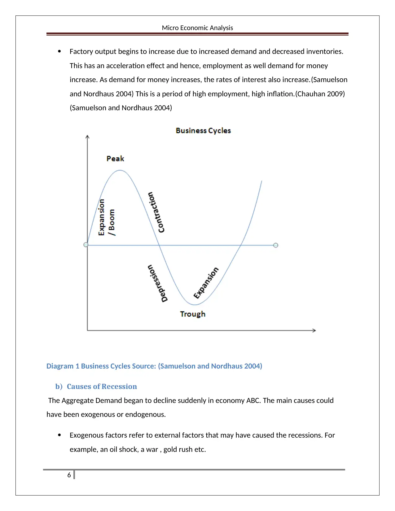
Factory output begins to increase due to increased demand and decreased inventories.
This has an acceleration effect and hence, employment as well demand for money
increase. As demand for money increases, the rates of interest also increase.(Samuelson
and Nordhaus 2004) This is a period of high employment, high inflation.(Chauhan 2009)
(Samuelson and Nordhaus 2004)
Diagram 1 Business Cycles Source: (Samuelson and Nordhaus 2004)
b) Causes of Recession
The Aggregate Demand began to decline suddenly in economy ABC. The main causes could
have been exogenous or endogenous.
Exogenous factors refer to external factors that may have caused the recessions. For
example, an oil shock, a war , gold rush etc.
6
⊘ This is a preview!⊘
Do you want full access?
Subscribe today to unlock all pages.
Trusted by 1+ million students worldwide
Micro Economic Analysis
Endogenous factors refer to the mechanism within the economy that may have caused the
recession.(Samuelson and Nordhaus 2004) Endogenous factors could be related to the supply
side of the economy or the demand side of the economy. However, the given example refers to
a decrease in aggregate demand and not a supply side decrease in output.
Monetary theorists often attribute such decrease in the demand to fluctuations in credit and
money supply. The multiplier effect of A typical case of such a recession begins when there is a
tight money policy or low government or private spending in the economy. (Samuelson and
Nordhaus 2004)
In the given example of country ABC, there is no reference to any external shock .Hence, the
factors in the given example would have been endogenous factors.
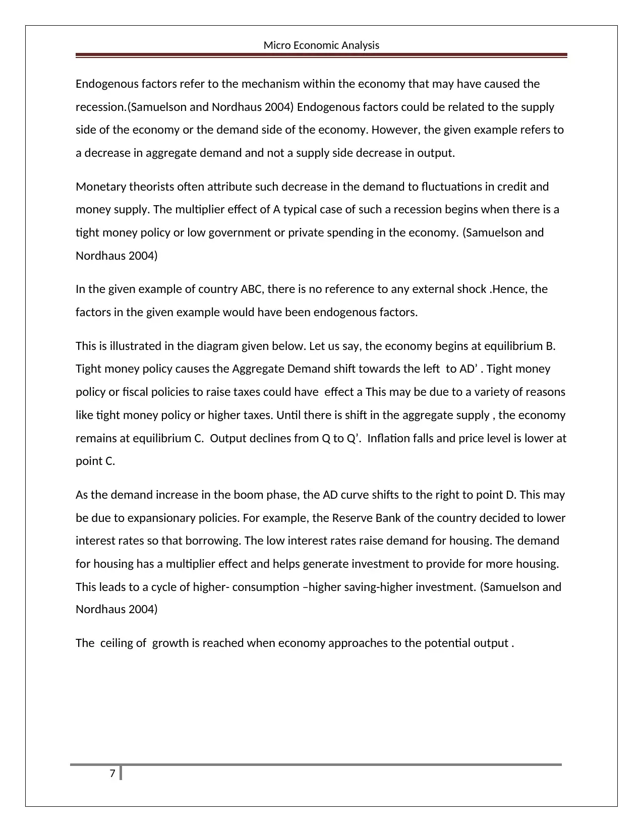
This is illustrated in the diagram given below. Let us say, the economy begins at equilibrium B.
Tight money policy causes the Aggregate Demand shift towards the left to AD’ . Tight money
policy or fiscal policies to raise taxes could have effect a This may be due to a variety of reasons
like tight money policy or higher taxes. Until there is shift in the aggregate supply , the economy
remains at equilibrium C. Output declines from Q to Q’. Inflation falls and price level is lower at
point C.
As the demand increase in the boom phase, the AD curve shifts to the right to point D. This may
be due to expansionary policies. For example, the Reserve Bank of the country decided to lower
interest rates so that borrowing. The low interest rates raise demand for housing. The demand
for housing has a multiplier effect and helps generate investment to provide for more housing.
This leads to a cycle of higher- consumption –higher saving-higher investment. (Samuelson and
Nordhaus 2004)
The ceiling of growth is reached when economy approaches to the potential output .
7
Endogenous factors refer to the mechanism within the economy that may have caused the
recession.(Samuelson and Nordhaus 2004) Endogenous factors could be related to the supply
side of the economy or the demand side of the economy. However, the given example refers to
a decrease in aggregate demand and not a supply side decrease in output.
Monetary theorists often attribute such decrease in the demand to fluctuations in credit and
money supply. The multiplier effect of A typical case of such a recession begins when there is a
tight money policy or low government or private spending in the economy. (Samuelson and
Nordhaus 2004)
In the given example of country ABC, there is no reference to any external shock .Hence, the
factors in the given example would have been endogenous factors.
This is illustrated in the diagram given below. Let us say, the economy begins at equilibrium B.
Tight money policy causes the Aggregate Demand shift towards the left to AD’ . Tight money
policy or fiscal policies to raise taxes could have effect a This may be due to a variety of reasons
like tight money policy or higher taxes. Until there is shift in the aggregate supply , the economy
remains at equilibrium C. Output declines from Q to Q’. Inflation falls and price level is lower at
point C.
As the demand increase in the boom phase, the AD curve shifts to the right to point D. This may
be due to expansionary policies. For example, the Reserve Bank of the country decided to lower
interest rates so that borrowing. The low interest rates raise demand for housing. The demand
for housing has a multiplier effect and helps generate investment to provide for more housing.
This leads to a cycle of higher- consumption –higher saving-higher investment. (Samuelson and
Nordhaus 2004)
The ceiling of growth is reached when economy approaches to the potential output .
7
Paraphrase This Document
Need a fresh take? Get an instant paraphrase of this document with our AI Paraphraser
Micro Economic Analysis
Diagram 2 Demand Side Illustration of Recession and Expansion. Source: (Samuelson and
Nordhaus 2004) Adapted by Author
Case 2
a) In 2001, the consumers have 3 choices: Britannica Book set, Britannica CD, Encarta CD.
In order to answer this question, the following assumptions must be made:
o Consumers definitely choose to buy at least one product.
o Price is the only determinant of choice
o Consumers are indifferent to the three choices, I.e. tastes and preferences are
not counted
Substitutability between Britannica Book set and Britannica CD. Given a choice in
2001, the consumer could purchase the Encarta CD instead of the Book Set
because the Encarta CD is the second best choice based on price. Hence, the two
8
Micro Economic Analysis
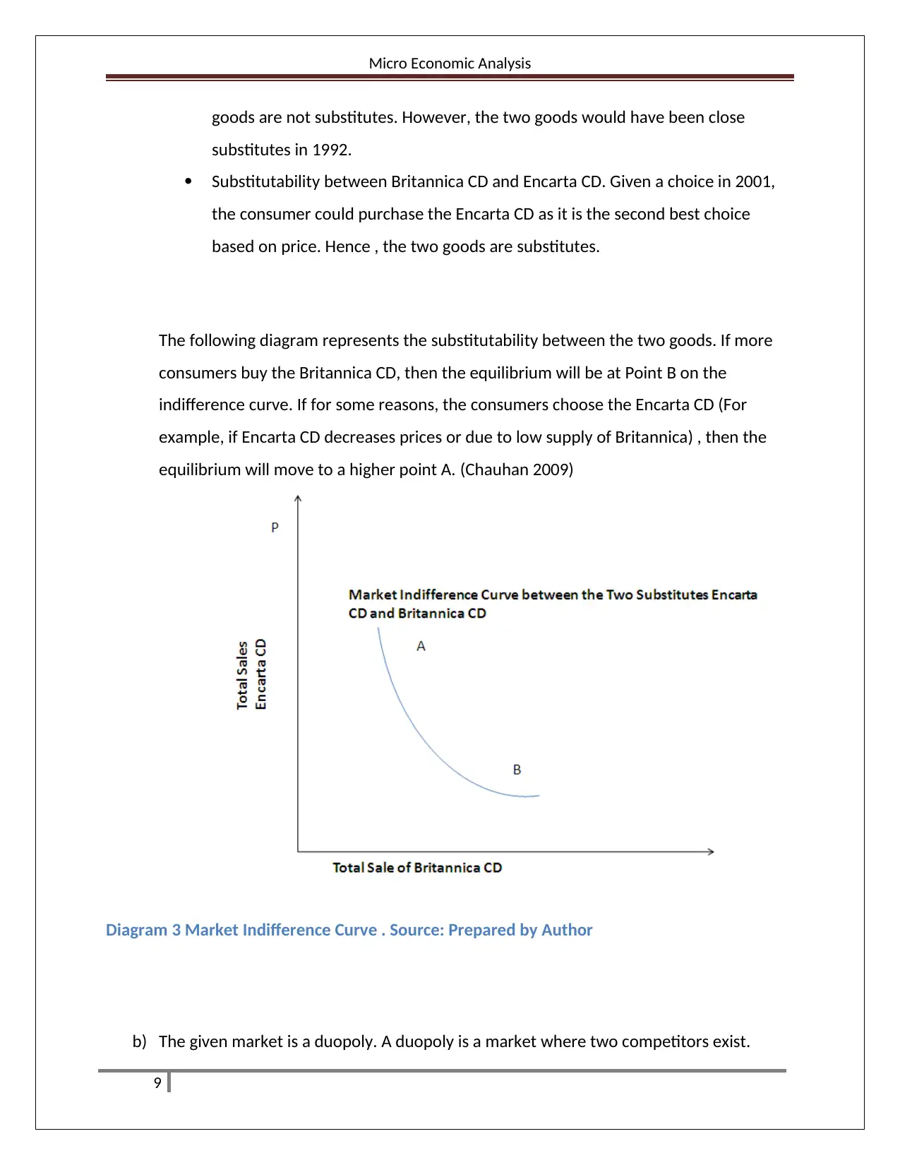
goods are not substitutes. However, the two goods would have been close
substitutes in 1992.
Substitutability between Britannica CD and Encarta CD. Given a choice in 2001,
the consumer could purchase the Encarta CD as it is the second best choice
based on price. Hence , the two goods are substitutes.
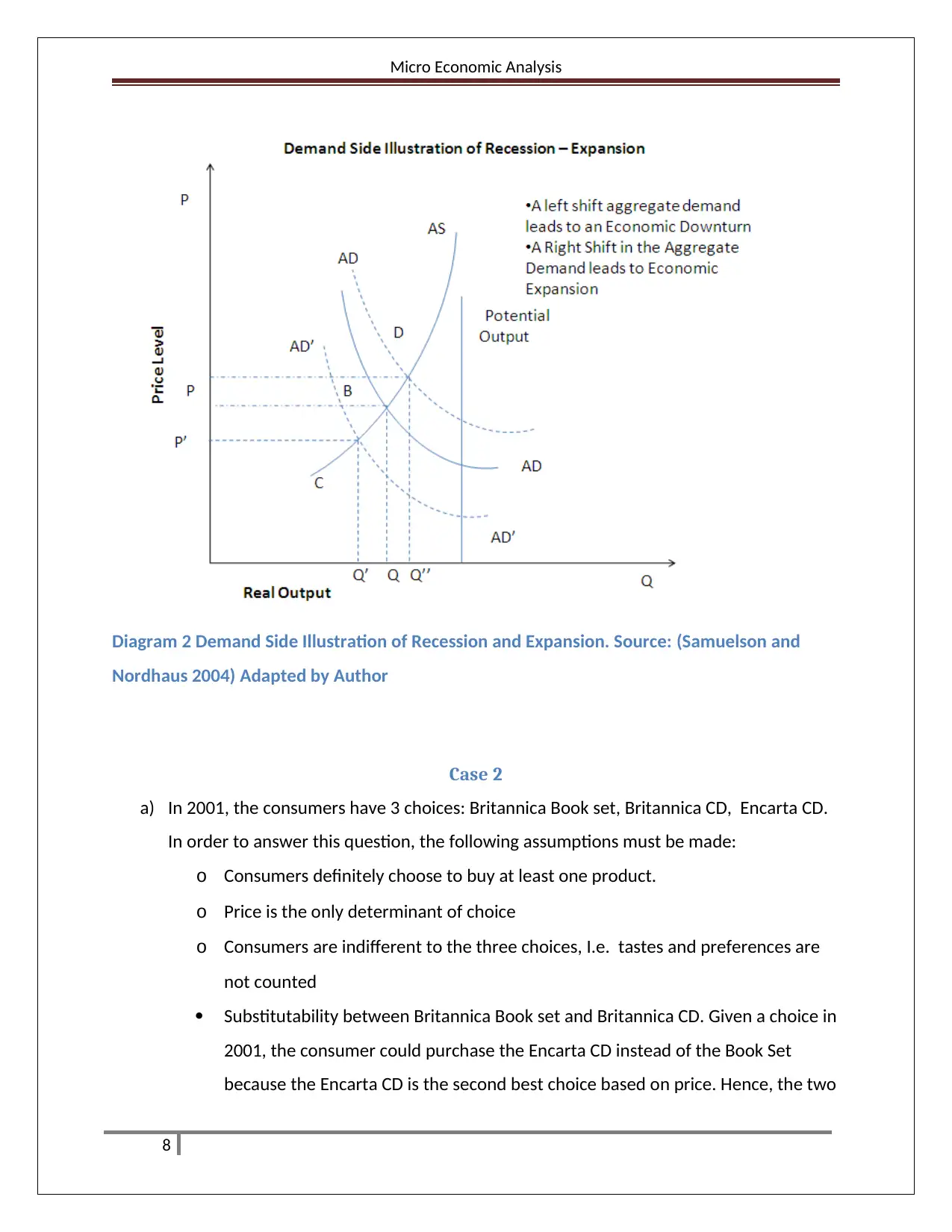
The following diagram represents the substitutability between the two goods. If more
consumers buy the Britannica CD, then the equilibrium will be at Point B on the
indifference curve. If for some reasons, the consumers choose the Encarta CD (For
example, if Encarta CD decreases prices or due to low supply of Britannica) , then the
equilibrium will move to a higher point A. (Chauhan 2009)
Diagram 3 Market Indifference Curve . Source: Prepared by Author
b) The given market is a duopoly. A duopoly is a market where two competitors exist.
9
goods are not substitutes. However, the two goods would have been close
substitutes in 1992.
Substitutability between Britannica CD and Encarta CD. Given a choice in 2001,
the consumer could purchase the Encarta CD as it is the second best choice
based on price. Hence , the two goods are substitutes.
The following diagram represents the substitutability between the two goods. If more
consumers buy the Britannica CD, then the equilibrium will be at Point B on the
indifference curve. If for some reasons, the consumers choose the Encarta CD (For
example, if Encarta CD decreases prices or due to low supply of Britannica) , then the
equilibrium will move to a higher point A. (Chauhan 2009)
Diagram 3 Market Indifference Curve . Source: Prepared by Author
b) The given market is a duopoly. A duopoly is a market where two competitors exist.
9
⊘ This is a preview!⊘
Do you want full access?
Subscribe today to unlock all pages.
Trusted by 1+ million students worldwide

Micro Economic Analysis
In such a market, best decisions would be made keeping in mind not just the consumer
demand but also the strategy or the game expected to be played by the competitor.
In order to maximize revenues, it would be best to take the decision based on Game
Theory. (Samuelson and Nordhaus 2004)
Game Theory describes a series of strategy decisions taken by different sellers to maximize
their ‘profit’ or pay-of . These decisions affect all parties and decisions are often met with
retaliatory actions. (Samuelson and Nordhaus 2004)
According to the Theory, pay-offs will be maximized if both parties can collude. Collusion would
lead to both sellers earning monopoly profits by allowing them to act as one seller with a
monopoly price. Hence, the best decisions for the firms would be to collude at $200.
Competitive games would come into play , if Microsoft refuses to collude.
Since a price war would come into play, Microsoft may choose to reduce prices to $49.95.
Micro-soft also has marketing channels. The price of $49.95 should be considered as a low price
since the profit margins will be low. Hence, the firm should engage in non-price competition
and seeking marketing channels like exclusive deals with academic institutions.
The books would still be sold as a premium product since the book set and the CD are not
substitutes. Some non-price competition measures would be
Providing a Britannica CD free of cost with every Book set
Seeking to partner with exclusive customers
Advertising etc.
Assuming that Microsoft does not lower prices , in retaliation. It will lose market share and
hence, must engage in non-price competition mention above. In such a situation, Britannica can
set the price at $74.95
Table 1 Pay-off Matrix in Case of Strategic Games
Source: Prepared by Student
10
Paraphrase This Document
Need a fresh take? Get an instant paraphrase of this document with our AI Paraphraser
Micro Economic Analysis
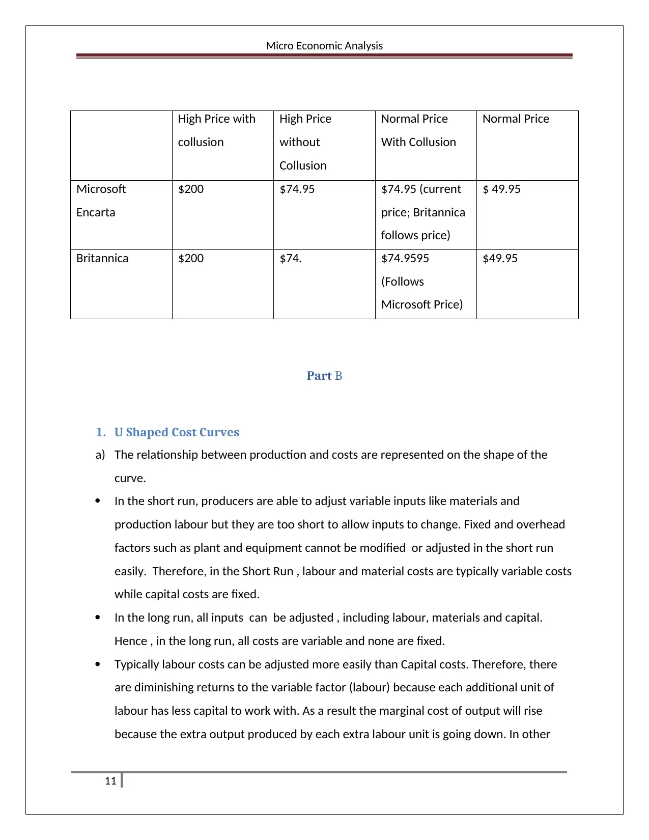
High Price with
collusion
High Price
without
Collusion
Normal Price
With Collusion
Normal Price
Microsoft
Encarta
$200 $74.95 $74.95 (current
price; Britannica
follows price)
$ 49.95
Britannica $200 $74. $74.9595
(Follows
Microsoft Price)
$49.95
Part B
1. U Shaped Cost Curves
a) The relationship between production and costs are represented on the shape of the
curve.
In the short run, producers are able to adjust variable inputs like materials and
production labour but they are too short to allow inputs to change. Fixed and overhead
factors such as plant and equipment cannot be modified or adjusted in the short run
easily. Therefore, in the Short Run , labour and material costs are typically variable costs
while capital costs are fixed.
In the long run, all inputs can be adjusted , including labour, materials and capital.
Hence , in the long run, all costs are variable and none are fixed.
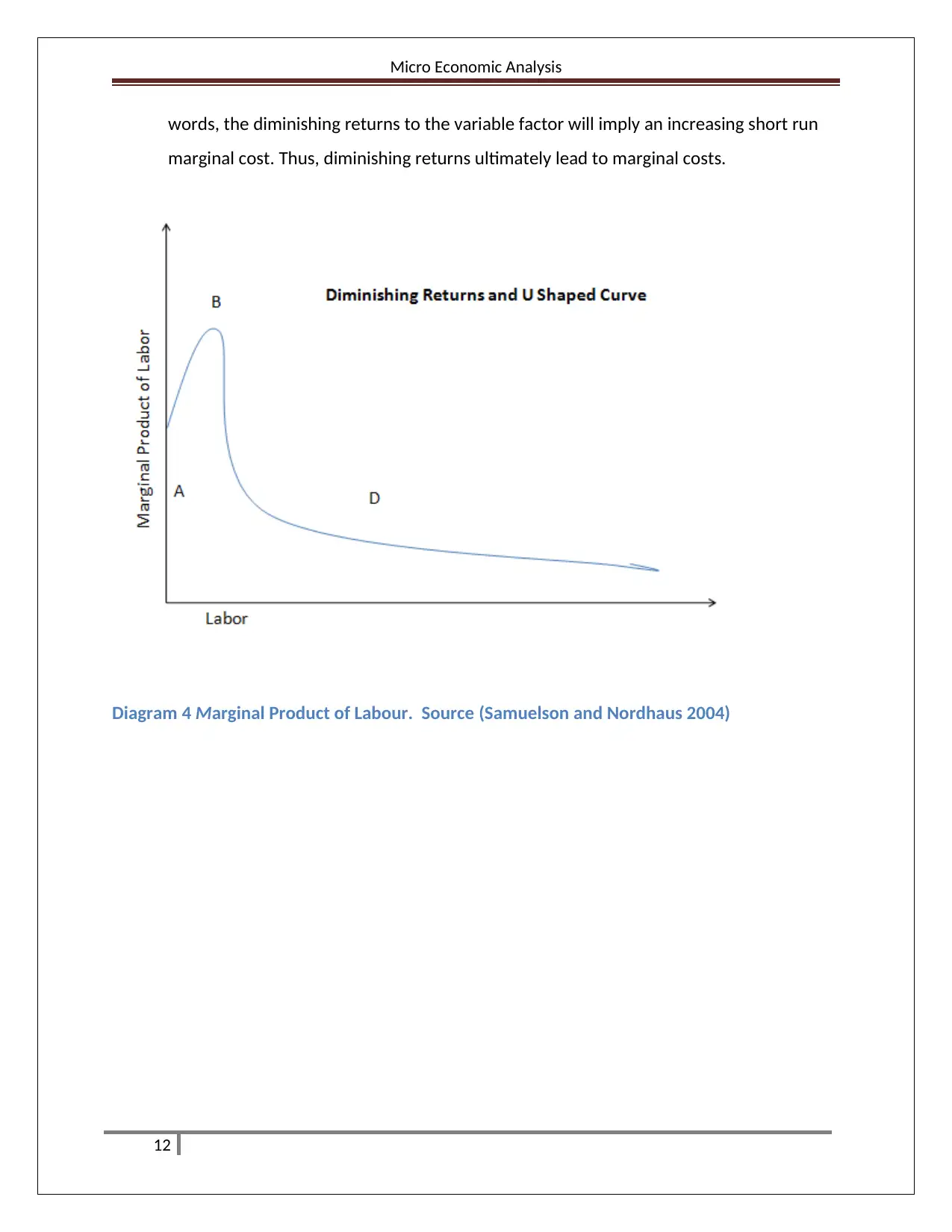
Typically labour costs can be adjusted more easily than Capital costs. Therefore, there
are diminishing returns to the variable factor (labour) because each additional unit of
labour has less capital to work with. As a result the marginal cost of output will rise
because the extra output produced by each extra labour unit is going down. In other
11
High Price with
collusion
High Price
without
Collusion
Normal Price
With Collusion
Normal Price
Microsoft
Encarta
$200 $74.95 $74.95 (current
price; Britannica
follows price)
$ 49.95
Britannica $200 $74. $74.9595
(Follows
Microsoft Price)
$49.95
Part B
1. U Shaped Cost Curves
a) The relationship between production and costs are represented on the shape of the
curve.
In the short run, producers are able to adjust variable inputs like materials and
production labour but they are too short to allow inputs to change. Fixed and overhead
factors such as plant and equipment cannot be modified or adjusted in the short run
easily. Therefore, in the Short Run , labour and material costs are typically variable costs
while capital costs are fixed.
In the long run, all inputs can be adjusted , including labour, materials and capital.
Hence , in the long run, all costs are variable and none are fixed.
Typically labour costs can be adjusted more easily than Capital costs. Therefore, there
are diminishing returns to the variable factor (labour) because each additional unit of
labour has less capital to work with. As a result the marginal cost of output will rise
because the extra output produced by each extra labour unit is going down. In other
11
Micro Economic Analysis
words, the diminishing returns to the variable factor will imply an increasing short run
marginal cost. Thus, diminishing returns ultimately lead to marginal costs.
Diagram 4 Marginal Product of Labour. Source (Samuelson and Nordhaus 2004)
12
words, the diminishing returns to the variable factor will imply an increasing short run
marginal cost. Thus, diminishing returns ultimately lead to marginal costs.
Diagram 4 Marginal Product of Labour. Source (Samuelson and Nordhaus 2004)
12
⊘ This is a preview!⊘
Do you want full access?
Subscribe today to unlock all pages.
Trusted by 1+ million students worldwide
1 out of 27
Related Documents


Your All-in-One AI-Powered Toolkit for Academic Success.
+13062052269
info@desklib.com
Available 24*7 on WhatsApp / Email
![[object Object]](/_next/static/media/star-bottom.7253800d.svg)
Unlock your academic potential
Copyright © 2020–2026 A2Z Services. All Rights Reserved. Developed and managed by ZUCOL.