Microeconomics Assignment: Market Structures, Elasticity, and Welfare

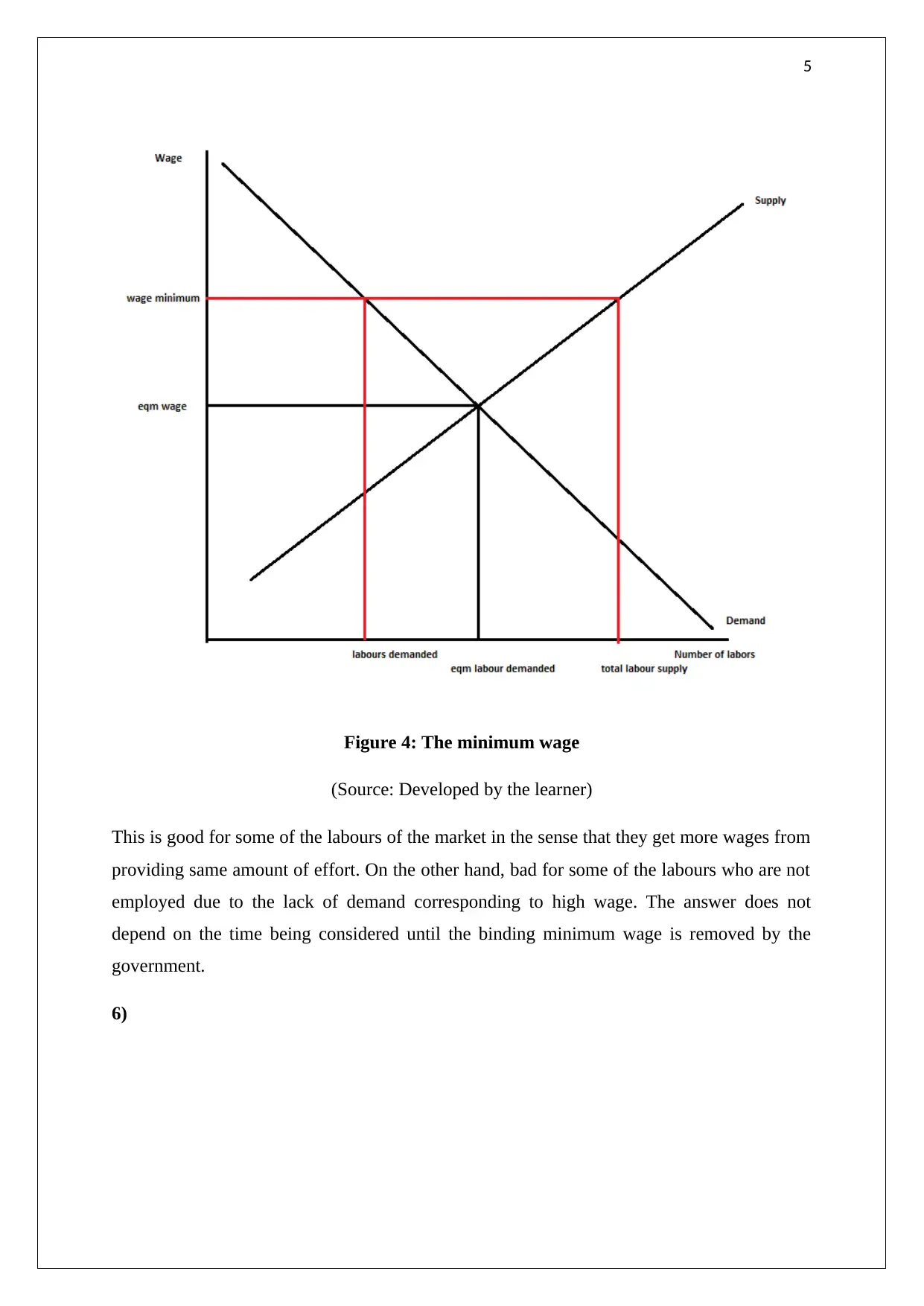
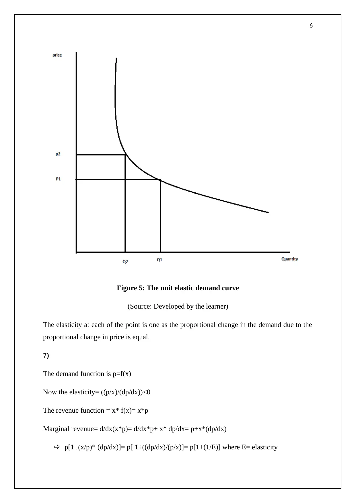
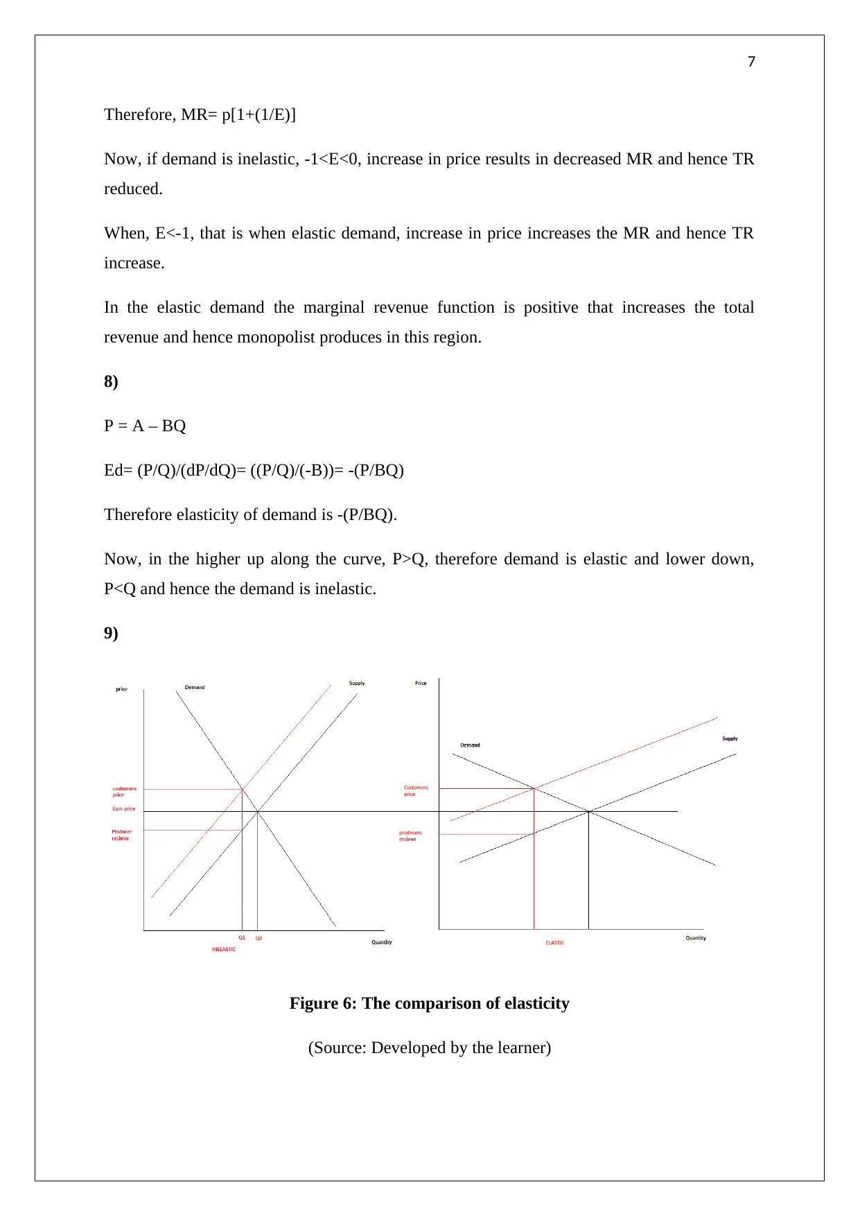
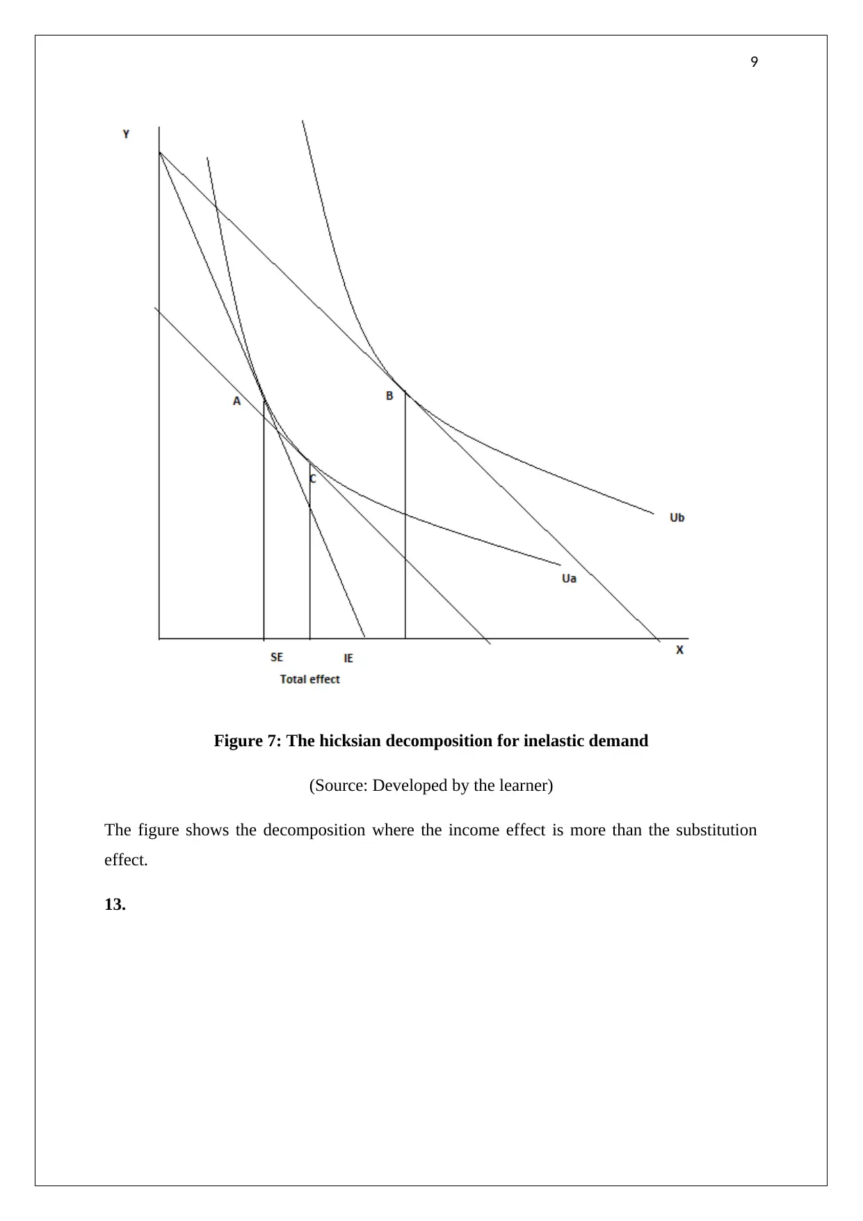
This microeconomics assignment solution covers a wide range of topics, including demand and supply functions, inverse demand and supply curves, and the impact of changes in marginal costs on market equilibrium. It explores the concept of complements, minimum wage effects, and the unit elastic demand curve. The assignment delves into elasticity, marginal revenue, and total revenue relationships, along with graphical representations. It also includes indifference curves, Hicksian decomposition, and the concept of present value of utility. The assignment explores production costs, returns to scale, and the relationship between long-run and short-run average cost curves. Furthermore, it examines profit maximization under perfect competition and monopoly, market structures, Herfindahl-Hirschman Index, Cournot Nash equilibrium, monopolistic competition, consumer and producer surplus, welfare loss, and the provision of public goods. The solution provides detailed explanations and graphical analyses for each question.

1
MICROECONOMICS ASSIGNMENT

2
Questions
1)
Figure 1: The demand and change in demand
(Source: Developed by the learner)
The demand function is Q=a+bP whereas the inverse demand curve is P=(Q-a)/b
While demand function determines quantity corresponding to price, the inverse demand
determines the price corresponding to quantity. Therefore, both these help in determining the
shape of the demand curve. When there is a change in the demand the value of the Q changes
keeping the value of P constant.
2)

3
Figure 2: The supply curve
(Source: Developed by the learner)
The supply curve is Q=c+dP and inverse supply is P=(Q-c)/d
Both the firm captures the change in one variable to the other giving the shape of the supply
curve. In case of the change in supply, Q changes with an unchanged level of price.
3)

4
Figure 3: The increase in the marginal cost
(Source: Developed by the learner)
Increase in the marginal cost increases the average cost and hence the supply curve shifts to
the left side in the market. The resultant equilibrium changes to a higher price and lower
quantity sold.
4)
For this definition to be accurate the other factors such as the income of the consumer,
changes in tastes and preferences needs to be unchanged.
5)

5
Figure 4: The minimum wage
(Source: Developed by the learner)
This is good for some of the labours of the market in the sense that they get more wages from
providing same amount of effort. On the other hand, bad for some of the labours who are not
employed due to the lack of demand corresponding to high wage. The answer does not
depend on the time being considered until the binding minimum wage is removed by the
government.
6)

6
Figure 5: The unit elastic demand curve
(Source: Developed by the learner)
The elasticity at each of the point is one as the proportional change in the demand due to the
proportional change in price is equal.
7)
The demand function is p=f(x)
Now the elasticity= ((p/x)/(dp/dx))<0
The revenue function = x* f(x)= x*p
Marginal revenue= d/dx(x*p)= d/dx*p+ x* dp/dx= p+x*(dp/dx)
 p[1+(x/p)* (dp/dx)]= p[ 1+((dp/dx)/(p/x)]= p[1+(1/E)] where E= elasticity

7
Therefore, MR= p[1+(1/E)]
Now, if demand is inelastic, -1<E<0, increase in price results in decreased MR and hence TR
reduced.
When, E<-1, that is when elastic demand, increase in price increases the MR and hence TR
increase.
In the elastic demand the marginal revenue function is positive that increases the total
revenue and hence monopolist produces in this region.
8)
P = A – BQ
Ed= (P/Q)/(dP/dQ)= ((P/Q)/(-B))= -(P/BQ)
Therefore elasticity of demand is -(P/BQ).
Now, in the higher up along the curve, P>Q, therefore demand is elastic and lower down,
P<Q and hence the demand is inelastic.
9)
Figure 6: The comparison of elasticity
(Source: Developed by the learner)

8
The figure above shows that in case of the inelastic demand and supply the revenue of the
taxes are more as can be seen from the area of the rectangle.
10.
Along the indifference curve the utility is same therefore, ΔX*MUx=-ΔY*MUy
=> ΔX/ -ΔY= MUx/ MUy
ΔX/ -ΔY is the marginal rate of substitution hence,
MRS= MUx/ MUy
11.
In this case the elasticity of demand is infinity that means proportional change in the quantity
demanded corresponding to the price is infinity. Any change in the price, the demand will
reduce to zero for a horizontal PCC.
12.

9
Figure 7: The hicksian decomposition for inelastic demand
(Source: Developed by the learner)
The figure shows the decomposition where the income effect is more than the substitution
effect.
13.

10
Figure 8: decomposition in the case of no income effect
(Source: Developed by the learner)
The figure depicts the substitution effect which is also the total change in the demand
corresponding to the reduction in the price level.
14.
EU= 0.3*500+0.7*0= $ 150
EV= (0.7)*(500)= $350
UEV= 0.3(500-350)+0.7(0-350+500)
$150

11
The answer depends on the whether the individual is risk neutral, averse or loving as
insurance amount is not stated.
15. Present value of the utility of some future event is known as the utility of an event that
can happen in the future. For example if someone invest a lump sum money, the future utility
is discounted at specific rate and denoted as present utility of future event.
The discount rate is the investment rate of return that is incorporated for the calculation of the
net present value or the utility.
If the discount rate is high the present utility of future event is low and vice versa.
16.
As the number of labour is increased the productivity of the labours decreases and hence cost
of production rises after the effect of the diminishing returns to scale.
17.

12
Figure 9: The increasing returns to scale
(Source: Developed by the learner)
18.
Figure 10: The LRAC and SRACT curves
(Source: Developed by the learner)
19.
Π= TR-TC
Now FOC
d Π/dQ= MR-MC= 0
This is the first order condition.
SOC is d2 Π/dQ2 is the second order condition.
The first order condition determines the optimal point and the second order condition
determines whether the optimal is least or highest.

13
In case of the perfect competition, MR=MC and hence the profit curve is linear and
horizontal.
20.
This is due to the fact that all the products sold in the market are homogenous and any
increase in price reduces the demand to zero and the customer makes the purchase elsewhere.
Industry market demand takes into consideration the elasticity of the product as a whole and
hence relatively less elastic.
21.
Figure 11: The MC and the min AVC
(Source: Developed by the learner)
As the price reduces the firm supplies reduces following the MC until the min AVC, below
which the production of the company stops and hence it represents the supply curve of the
firm.

14
The perfectly inelastic portion of the supply curve at low prices is due to the law of
diminishing returns. After this point as the production increases the marginal cost increases.
22.
The $1 per unit tax increases the cost of the production and hence the firm supplies the same
unit of good at higher prices and hence the curves moves upward.
23.
Figure 12: The zero economic profit monopolist
(Source: Developed by the learner)

15
Figure 13: The profit curve
(Source: Developed by the learner)
24.
a)

16
Figure 14: Loss making monopolist
(Source: Developed by the learner)
The profit of the monopolist has been shown by the rectangle.
b)

17
Figure 15: The profit of price discriminating monopolist
(Source: Developed by the learner)
The profit of the firm in this case is the whole triangle under the demand curve and above the
SRMC.
25.
HHI is the Herfindahl-Hirschman Index which is used to measure the concentration of the
indsutry. That means a duopolistic market with two sellers would capture more market share
and hence the concentration will be high. For the duopoly the value of the index is expected
to be high.
26.

18
In the case of the duopoly, the cournot nash equilibrium for the duopoly is for the player to
collude and set the price where the individual output levels maximises the joint profit.
27.
In a monopolistic competition the goods or the services sold are not homogenous to each
other but slightly different. The advertisement increases the visibility of the products and
further increases the differences from the rival product of the market. This is helpful in
gaining loyal customer for the company.
28.
Monopolist maximises profit where MR=MC
Therefore, Revenue= 50Q-2Q^2
MR= 50-4Q
Equating,
50-4Q= 1
 Q= 12.5
The price= 25
In perfect competition P=MC= 10
The quantity would be= 20
Therefore deadweight loss = 1/2*((20-12.5)*(25-10))= 56.25
29.
1)
here the supply = demand
Therefore
5+2Q=50-Q
 Qe= 15

19
Putting Q,
Pe= 35.
The consumer surplus= ½*((50-35)*(15))= 112.5
The producers surplus= ½*(35-5)*(15)= 225
Therefore consumer surplus+ producers surplus= 337.5
2)
Figure 16: The welfare loss
(Source: Developed by the learner)
The red triangle shows the welfare loss if the $1 worth of negative externality is ignored.
30.

20
Figure 17: The welfare diagram of public good provision
(Source: Developed by the learner)