Microeconomics Assignment: Analyzing Profit Maximization (MR=MC)

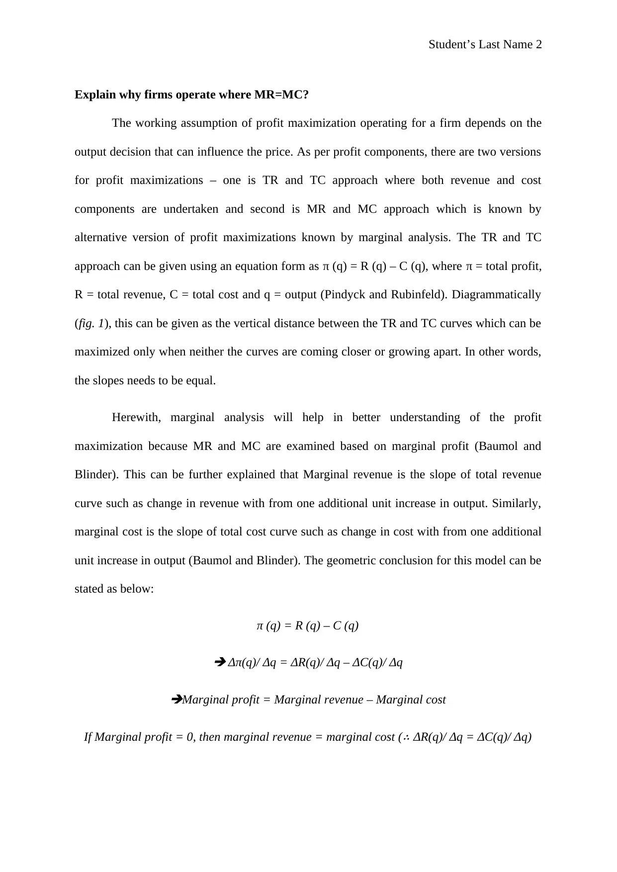
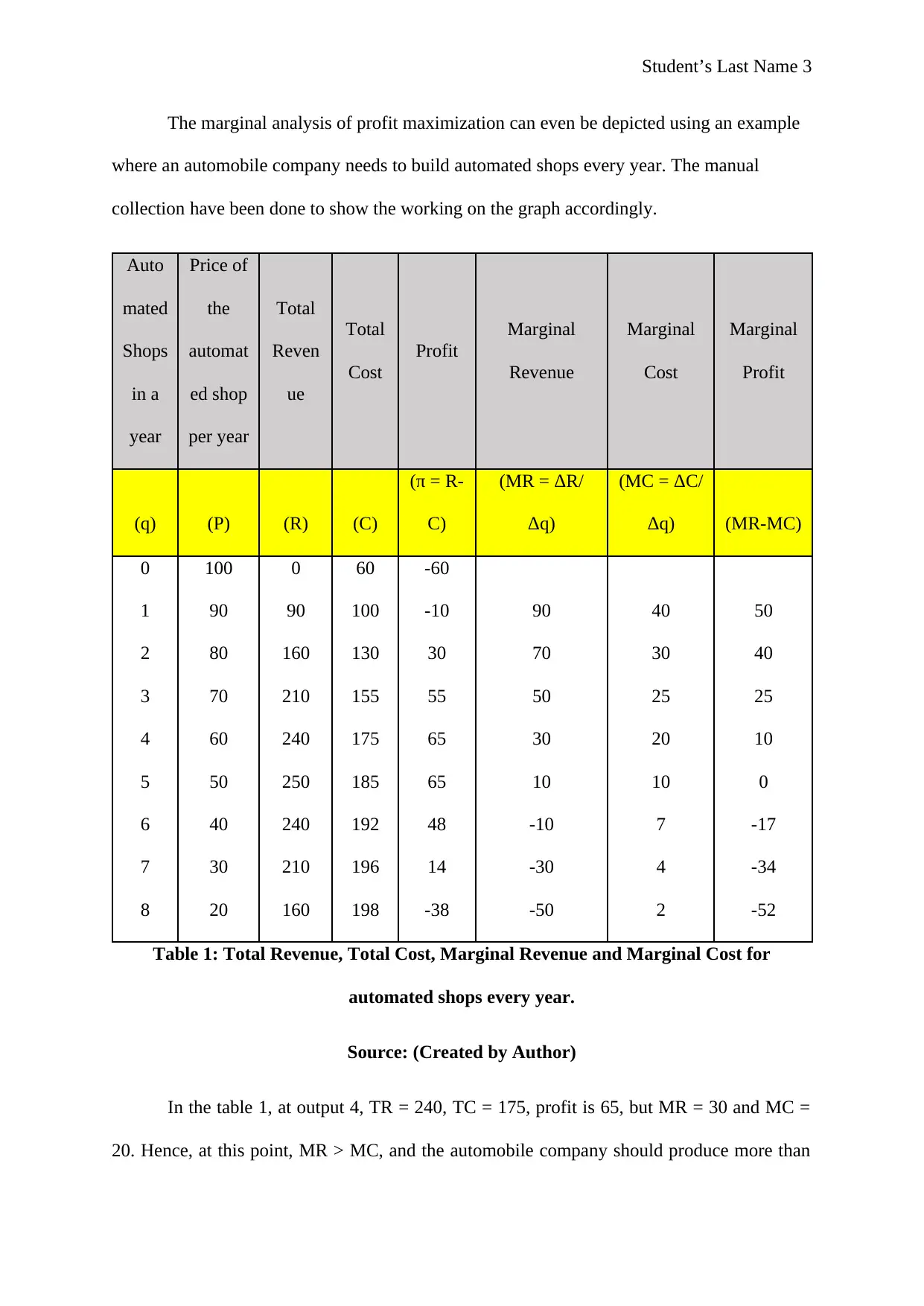
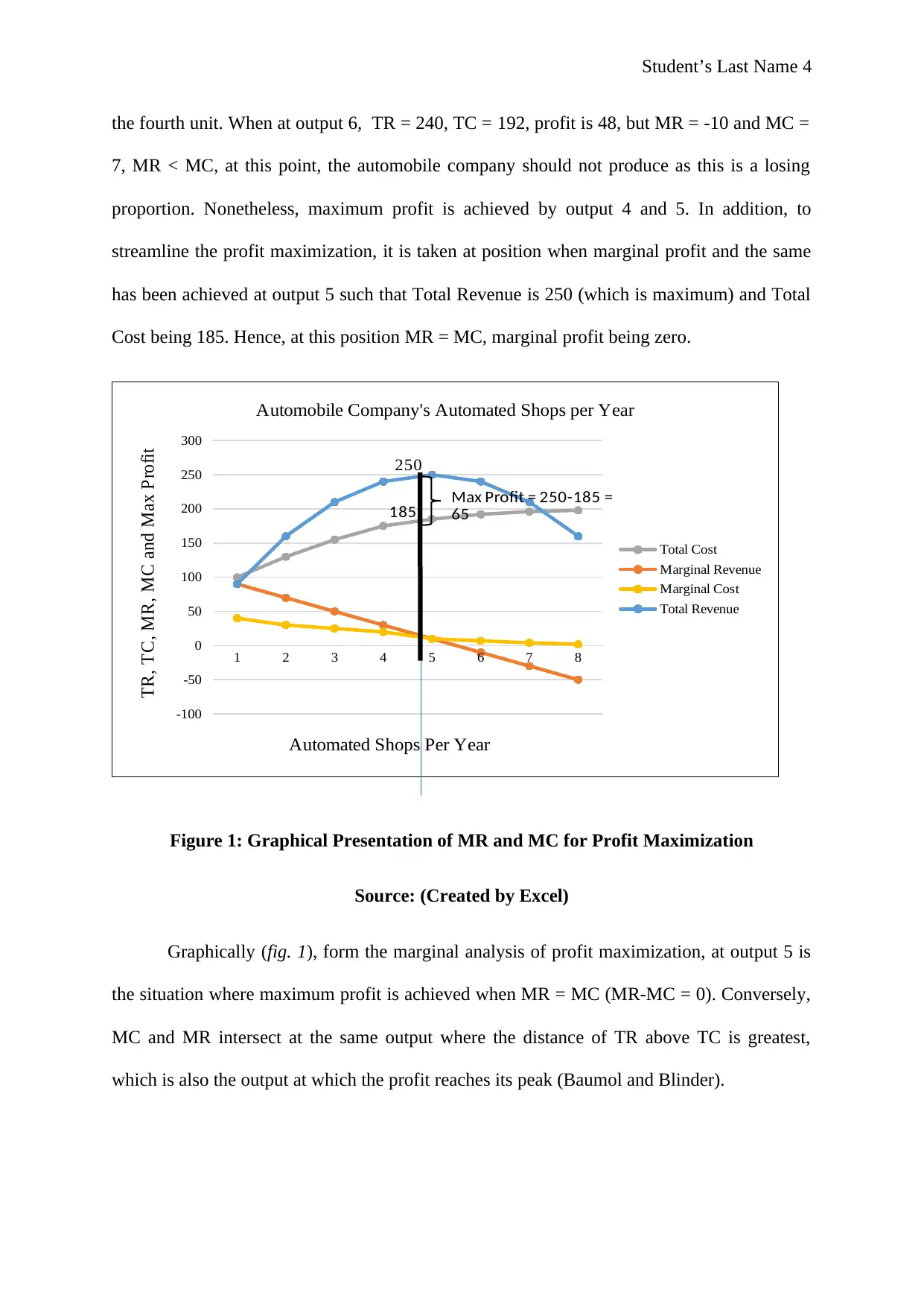
This microeconomics assignment explains the fundamental principle of profit maximization for firms, focusing on the condition where marginal revenue (MR) equals marginal cost (MC). The assignment utilizes both the total revenue and total cost approach, and the marginal analysis approach. The core argument is that firms maximize profit by producing at the output level where MR equals MC, as this point represents the greatest vertical distance between the total revenue and total cost curves. The assignment illustrates this concept with a numerical example of an automobile company's automated shops, providing a table of total revenue, total cost, marginal revenue, and marginal cost at different output levels, and a graphical representation of the MR and MC curves. The analysis demonstrates that the maximum profit is achieved when MR equals MC, and further explains that at this point, marginal profit is zero. The assignment concludes by referencing key economic literature supporting the analysis.

Running head: MICROECONOMICS
Name of the Student:
Class:
Date:

Student’s Last Name 2
Explain why firms operate where MR=MC?
The working assumption of profit maximization operating for a firm depends on the
output decision that can influence the price. As per profit components, there are two versions
for profit maximizations – one is TR and TC approach where both revenue and cost
components are undertaken and second is MR and MC approach which is known by
alternative version of profit maximizations known by marginal analysis. The TR and TC
approach can be given using an equation form as π (q) = R (q) – C (q), where π = total profit,
R = total revenue, C = total cost and q = output (Pindyck and Rubinfeld). Diagrammatically
(fig. 1), this can be given as the vertical distance between the TR and TC curves which can be
maximized only when neither the curves are coming closer or growing apart. In other words,
the slopes needs to be equal.
Herewith, marginal analysis will help in better understanding of the profit
maximization because MR and MC are examined based on marginal profit (Baumol and
Blinder). This can be further explained that Marginal revenue is the slope of total revenue
curve such as change in revenue with from one additional unit increase in output. Similarly,
marginal cost is the slope of total cost curve such as change in cost with from one additional
unit increase in output (Baumol and Blinder). The geometric conclusion for this model can be
stated as below:
π (q) = R (q) – C (q)
 Δπ(q)/ Δq = ΔR(q)/ Δq – ΔC(q)/ Δq
Marginal profit = Marginal revenue – Marginal cost
If Marginal profit = 0, then marginal revenue = marginal cost (
∴ ΔR(q)/ Δq = ΔC(q)/ Δq)

Student’s Last Name 3
The marginal analysis of profit maximization can even be depicted using an example
where an automobile company needs to build automated shops every year. The manual
collection have been done to show the working on the graph accordingly.
Auto
mated
Shops
in a
year
Price of
the
automat
ed shop
per year
Total
Reven
ue
Total
Cost
Profit
Marginal
Revenue
Marginal
Cost
Marginal
Profit
(q) (P) (R) (C)
(π = R-
C)
(MR = ΔR/
Δq)
(MC = ΔC/
Δq) (MR-MC)
0 100 0 60 -60
1 90 90 100 -10 90 40 50
2 80 160 130 30 70 30 40
3 70 210 155 55 50 25 25
4 60 240 175 65 30 20 10
5 50 250 185 65 10 10 0
6 40 240 192 48 -10 7 -17
7 30 210 196 14 -30 4 -34
8 20 160 198 -38 -50 2 -52
Table 1: Total Revenue, Total Cost, Marginal Revenue and Marginal Cost for
automated shops every year.
Source: (Created by Author)
In the table 1, at output 4, TR = 240, TC = 175, profit is 65, but MR = 30 and MC =
20. Hence, at this point, MR > MC, and the automobile company should produce more than

Student’s Last Name 4
the fourth unit. When at output 6, TR = 240, TC = 192, profit is 48, but MR = -10 and MC =
7, MR < MC, at this point, the automobile company should not produce as this is a losing
proportion. Nonetheless, maximum profit is achieved by output 4 and 5. In addition, to
streamline the profit maximization, it is taken at position when marginal profit and the same
has been achieved at output 5 such that Total Revenue is 250 (which is maximum) and Total
Cost being 185. Hence, at this position MR = MC, marginal profit being zero.
1 2 3 4 5 6 7 8
-100
-50
0
50
100
150
200
250
300
Automobile Company's Automated Shops per Year
Total Cost
Marginal Revenue
Marginal Cost
Total Revenue
Automated Shops Per Year
TR, TC, MR, MC and Max Profit
250
185 Max Profit = 250-185 =
65
Figure 1: Graphical Presentation of MR and MC for Profit Maximization
Source: (Created by Excel)
Graphically (fig. 1), form the marginal analysis of profit maximization, at output 5 is
the situation where maximum profit is achieved when MR = MC (MR-MC = 0). Conversely,
MC and MR intersect at the same output where the distance of TR above TC is greatest,
which is also the output at which the profit reaches its peak (Baumol and Blinder).

Student’s Last Name 5
References
Baumol, William J., and Alan S. Blinder. Microeconomics: Principles and policy. Nelson
Education, 2015.
Pindyck, R. S., and D. L. Rubinfeld. "Microeconomics; Eight Edition, Global Edition."
(2015).