Economics Assignment for Microeconomics: Chicken Market Analysis

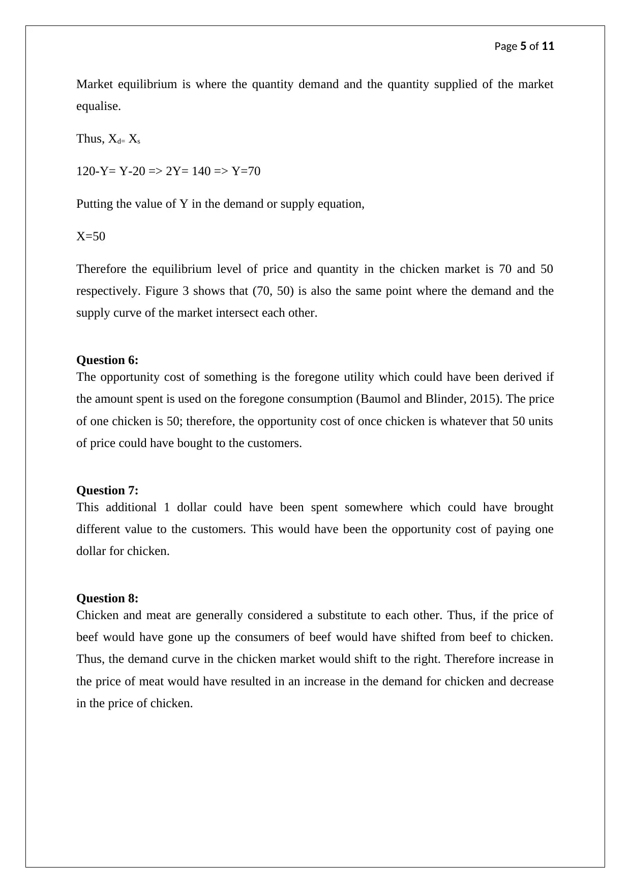
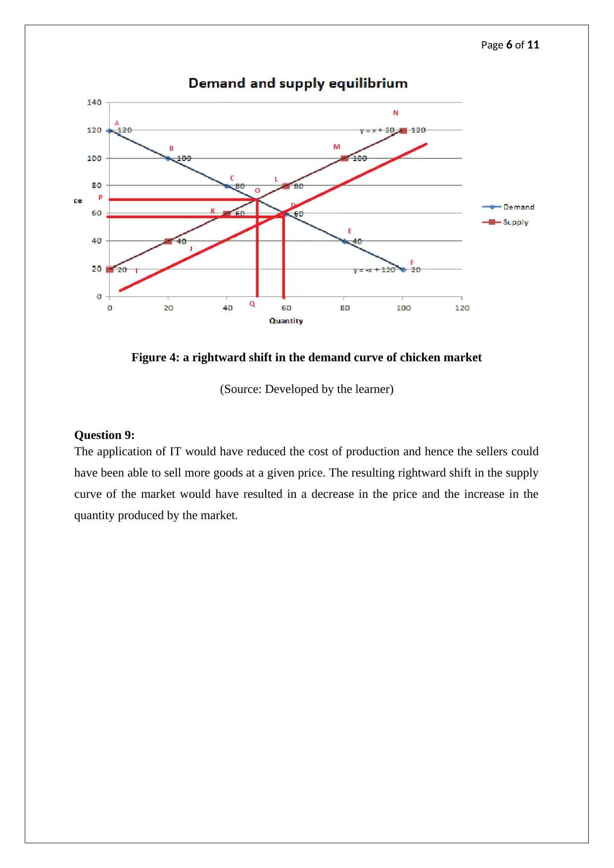
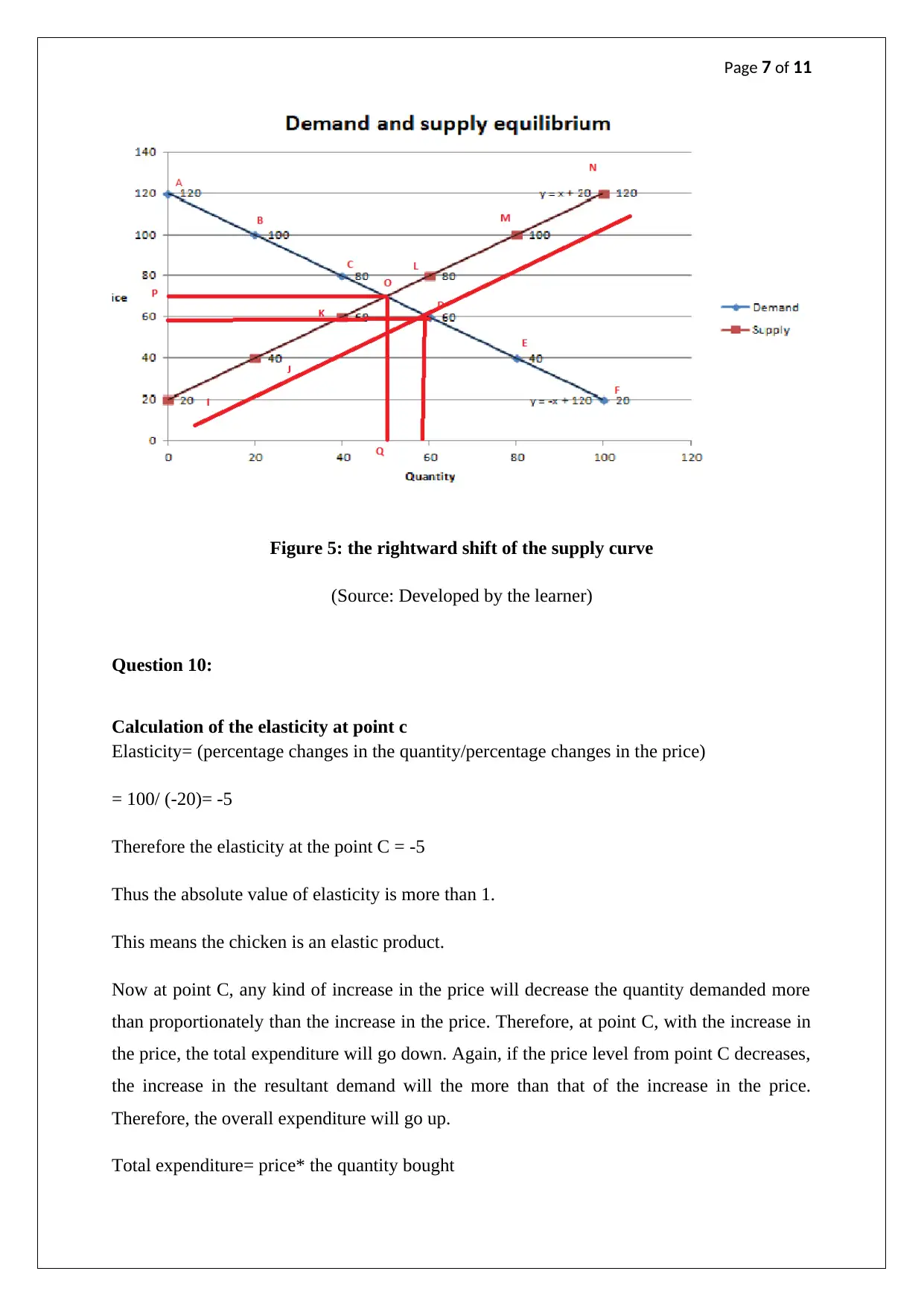
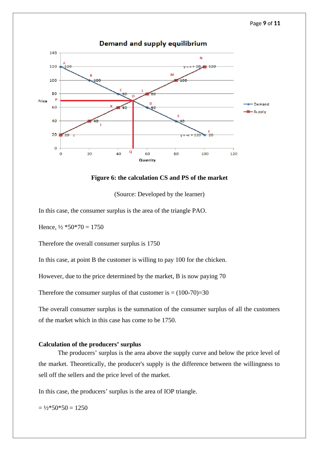
This microeconomics assignment analyzes the chicken market, exploring demand and supply curves, market equilibrium, and elasticity calculations. The assignment includes graphical representations of demand and supply, equations for demand and supply curves, and the determination of equilibrium price and quantity. It delves into the concept of opportunity cost and examines how changes in related goods (like beef) and technology impact the market. The solution calculates elasticity at a specific point, determining whether chicken is an elastic product. Furthermore, the assignment calculates and explains consumer and producer surplus, providing a comprehensive understanding of market dynamics. The document includes references to relevant economic literature.

Page 1 of 11
ECONOMICS ASSIGNMENT
ASSIGNMENT FOR MICROECONOMICS

Page 2 of 11
Table of contents
Question 1:.................................................................................................................................3
Question 2:.................................................................................................................................3
Question 3:.................................................................................................................................4
Question 4:.................................................................................................................................4
Question 5:.................................................................................................................................4
Question 6:.................................................................................................................................5
Question 7:.................................................................................................................................5
Question 8:.................................................................................................................................5
Question 9:.................................................................................................................................6
Question 10:...............................................................................................................................7
Calculation of the elasticity at point c........................................................................................7
Calculation of the elasticity of supply........................................................................................8
Calculation of the consumer surplus..........................................................................................8
Calculation of the producers’ surplus........................................................................................9
Reference..................................................................................................................................11

Page 3 of 11
Question 1:
0 20 40 60 80 100
0
20
40
60
80
100
120
140
Demand Curve
Demand Curve
Quantity
Price
Figure 1: The demand curve
(Source: Developed by the learner)
Question 2:
0 20 40 60 80 100
0
20
40
60
80
100
120
140
Suppy Curve
Suppy Curve
Quantity
Price
Figure 2: The supply curve
(Source: Developed by the learner)

Page 4 of 11
Question 3:
The demand curve equation for chicken is,
Y=120-X => Xd=120-Y
Where the Y= price of chicken
X= is the demand for chicken
Question 4:
The supply curve equation for chicken is,
Y=X+20 => Xs= Y-20
Where the Y= price of chicken
X= is the demand for chicken
Question 5:
0 20 40 60 80 100 120
0
20
40
60
80
100
120
140
20
40
60
80
100
120120
100
80
60
40
20
f(x) = x + 20f(x) = − x + 120
Demand and supply equilibrium
Demand
Linear (Demand)
Supply
Linear (Supply)
Quantity
Price
Figure 3: The demand and the supply equilibrium of the chicken market
(Source: Developed by the learner)

Page 5 of 11
Market equilibrium is where the quantity demand and the quantity supplied of the market
equalise.
Thus, Xd= Xs
120-Y= Y-20 => 2Y= 140 => Y=70
Putting the value of Y in the demand or supply equation,
X=50
Therefore the equilibrium level of price and quantity in the chicken market is 70 and 50
respectively. Figure 3 shows that (70, 50) is also the same point where the demand and the
supply curve of the market intersect each other.
Question 6:
The opportunity cost of something is the foregone utility which could have been derived if
the amount spent is used on the foregone consumption (Baumol and Blinder, 2015). The price
of one chicken is 50; therefore, the opportunity cost of once chicken is whatever that 50 units
of price could have bought to the customers.
Question 7:
This additional 1 dollar could have been spent somewhere which could have brought
different value to the customers. This would have been the opportunity cost of paying one
dollar for chicken.
Question 8:
Chicken and meat are generally considered a substitute to each other. Thus, if the price of
beef would have gone up the consumers of beef would have shifted from beef to chicken.
Thus, the demand curve in the chicken market would shift to the right. Therefore increase in
the price of meat would have resulted in an increase in the demand for chicken and decrease
in the price of chicken.

Page 6 of 11
Figure 4: a rightward shift in the demand curve of chicken market
(Source: Developed by the learner)
Question 9:
The application of IT would have reduced the cost of production and hence the sellers could
have been able to sell more goods at a given price. The resulting rightward shift in the supply
curve of the market would have resulted in a decrease in the price and the increase in the
quantity produced by the market.

Page 7 of 11
Figure 5: the rightward shift of the supply curve
(Source: Developed by the learner)
Question 10:
Calculation of the elasticity at point c
Elasticity= (percentage changes in the quantity/percentage changes in the price)
= 100/ (-20)= -5
Therefore the elasticity at the point C = -5
Thus the absolute value of elasticity is more than 1.
This means the chicken is an elastic product.
Now at point C, any kind of increase in the price will decrease the quantity demanded more
than proportionately than the increase in the price. Therefore, at point C, with the increase in
the price, the total expenditure will go down. Again, if the price level from point C decreases,
the increase in the resultant demand will the more than that of the increase in the price.
Therefore, the overall expenditure will go up.
Total expenditure= price* the quantity bought

Page 8 of 11
Price↑* quantity demanded ↓↓ = Total expenditure ↓↓
Price ↓ quantity demanded ↑↑= Total expenditure ↑↑
Calculation of the elasticity of supply
When the price moves from L to M there is a 25% increase in the price of chicken.
Now the resultant quantity supplied also increases by 33%
We know that the elasticity of supply= (percentage changes in the quantity supplied/
percentage changes in the price)
=33/25= +1.32
Therefore at point M, the elasticity of supply is +1.32.
This elasticity of supply is more than 1. That means with an increase in the price, the increase
in the quantity supplied is more than the increase in the price.
Now,
Total expenditure= price* the quantity bought
Price↑* quantity supplied ↑↑ = Total expenditure ↑↑
Price ↓ quantity demanded ↓↓= Total expenditure ↓↓
Calculation of the consumer surplus
As per the equilibrium of the market, (70, 50) is the point where the demand and the
supply curve of the market intersect with each other.
That means the price = 70 and quantity= 50
Now, consumer surplus is the area between the demand curve and the price level. In other
words, consumer surplus is the extra amount that the consumers are left with when the price
levels are lower than their respective reserve prices or willingness to pay (Goodwin et al.
2015).

Page 9 of 11
Figure 6: the calculation CS and PS of the market
(Source: Developed by the learner)
In this case, the consumer surplus is the area of the triangle PAO.
Hence, ½ *50*70 = 1750
Therefore the overall consumer surplus is 1750
In this case, at point B the customer is willing to pay 100 for the chicken.
However, due to the price determined by the market, B is now paying 70
Therefore the consumer surplus of that customer is = (100-70)=30
The overall consumer surplus is the summation of the consumer surplus of all the customers
of the market which in this case has come to be 1750.
Calculation of the producers’ surplus
The producers’ surplus is the area above the supply curve and below the price level of
the market. Theoretically, the producer's supply is the difference between the willingness to
sell off the sellers and the price level of the market.
In this case, the producers’ surplus is the area of IOP triangle.
= ½*50*50 = 1250

Page 10 of 11
Thus, the overall producers’ surplus is 1250.
In this case, the seller at point J is willing to sell his chicken at price level of 40
However, with the interaction of the demand and the supply curve of the market, the
equilibrium price is 70
Thus, the seller at point J is actually getting 70 instead of 40
The producers’ surplus at point J is = (70-40)= 30
The overall producers’ surplus of the market is the producers’ surplus of all the sellers which
in this case has come to be 1250.

Page 11 of 11
Reference
Baumol, W.J., and Blinder, A.S., 2015. Microeconomics: Principles and policy. Cengage
Learning.
Goodwin, N., Harris, J.M., Nelson, J.A., Roach, B. and Torras, M., 2015. Microeconomics in
context. Routledge.