Microeconomics Assignment: Production Possibility, Market Analysis

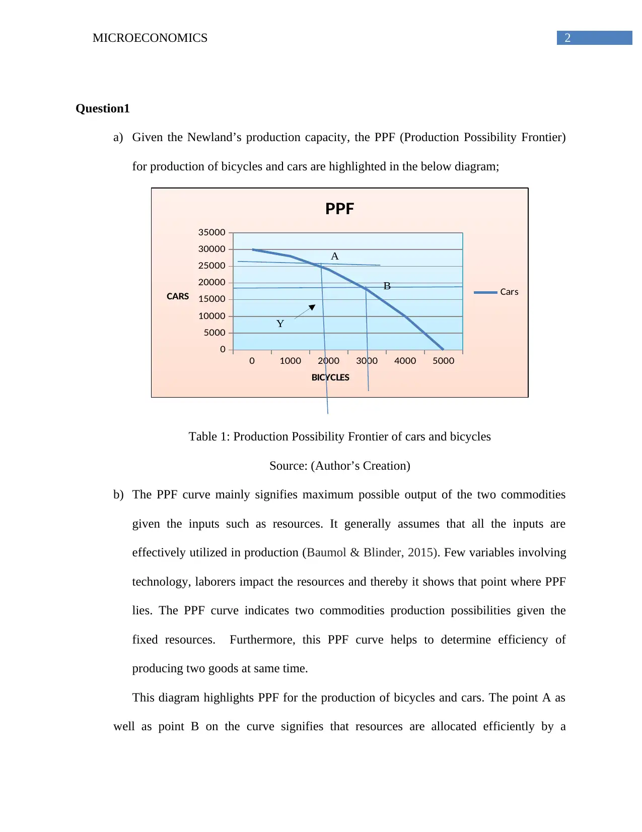
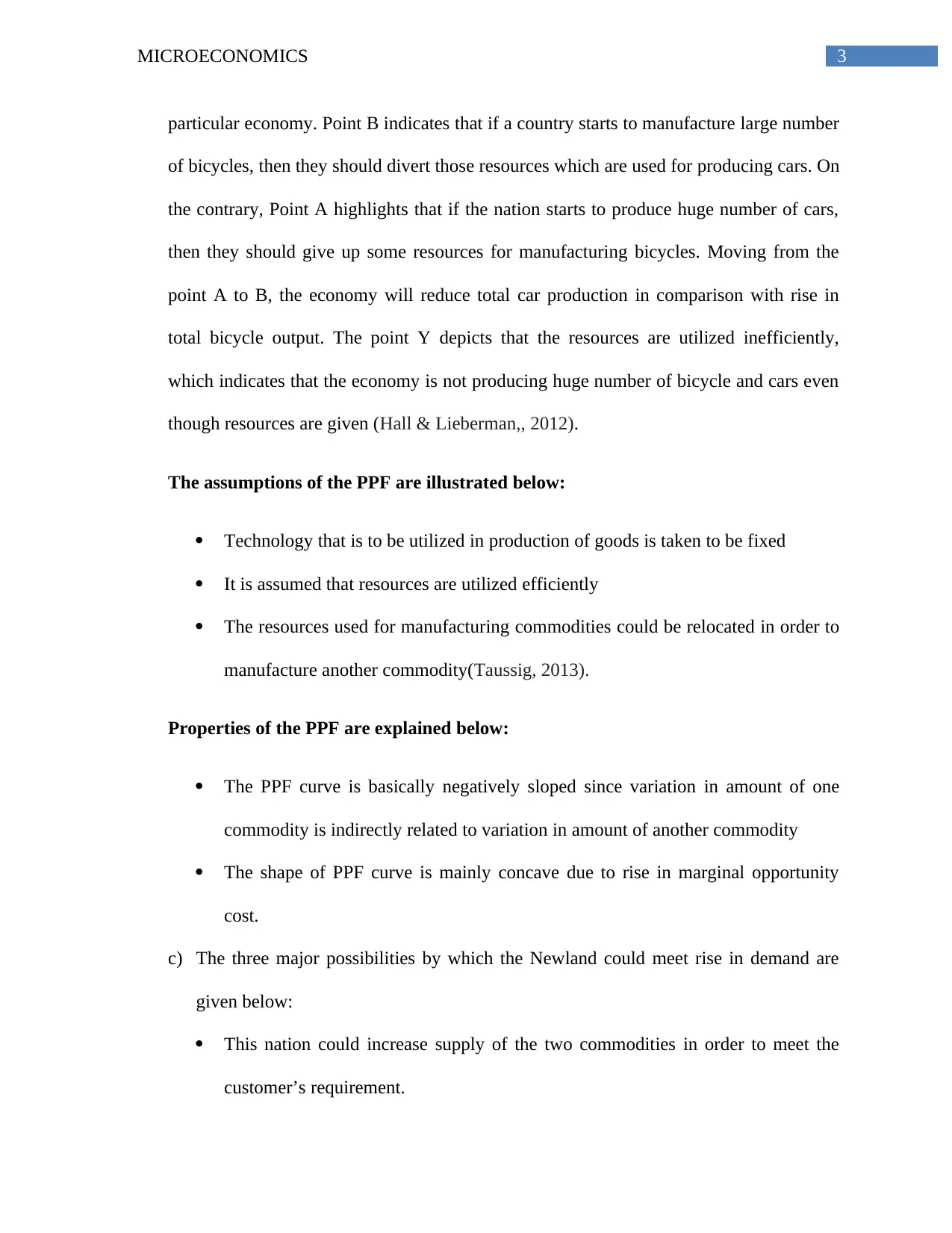
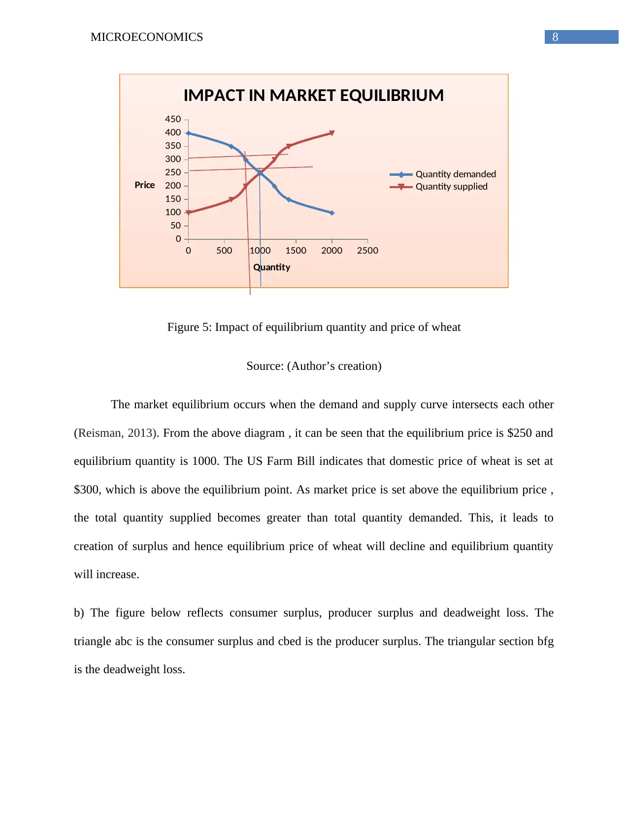
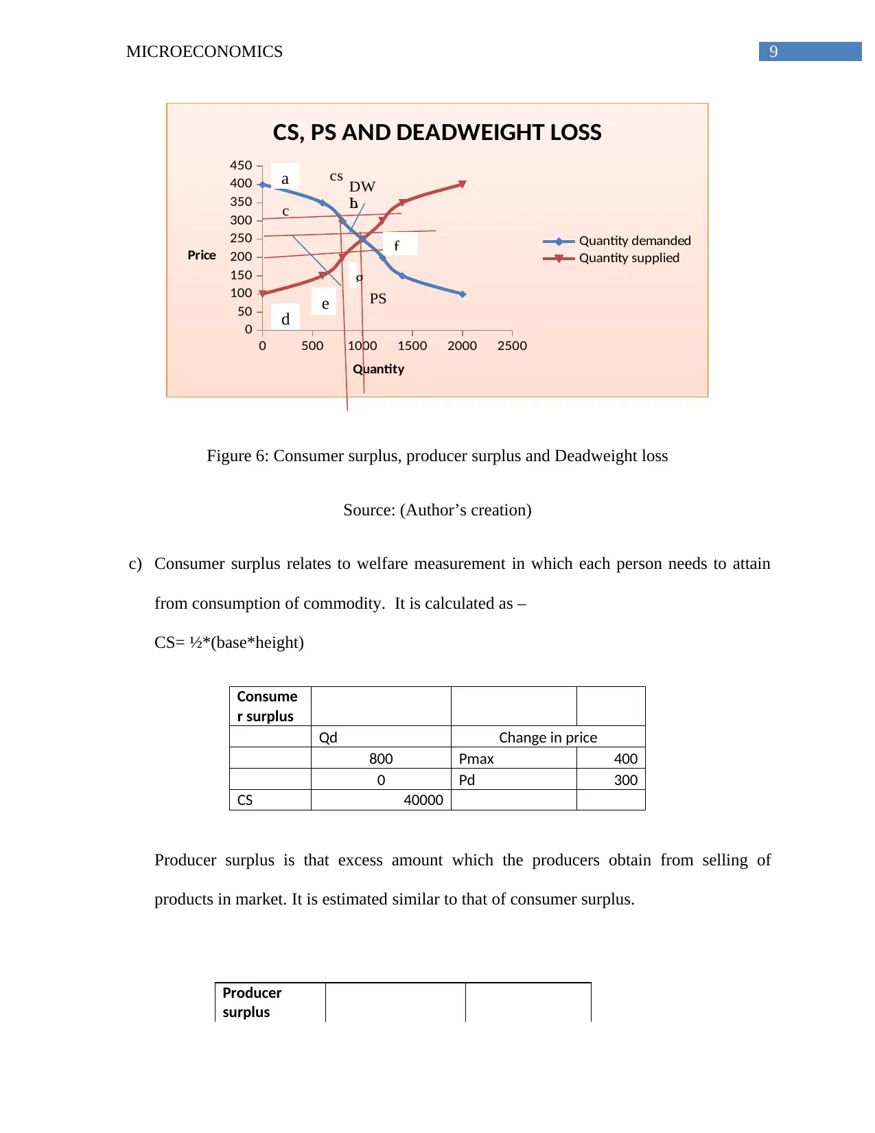
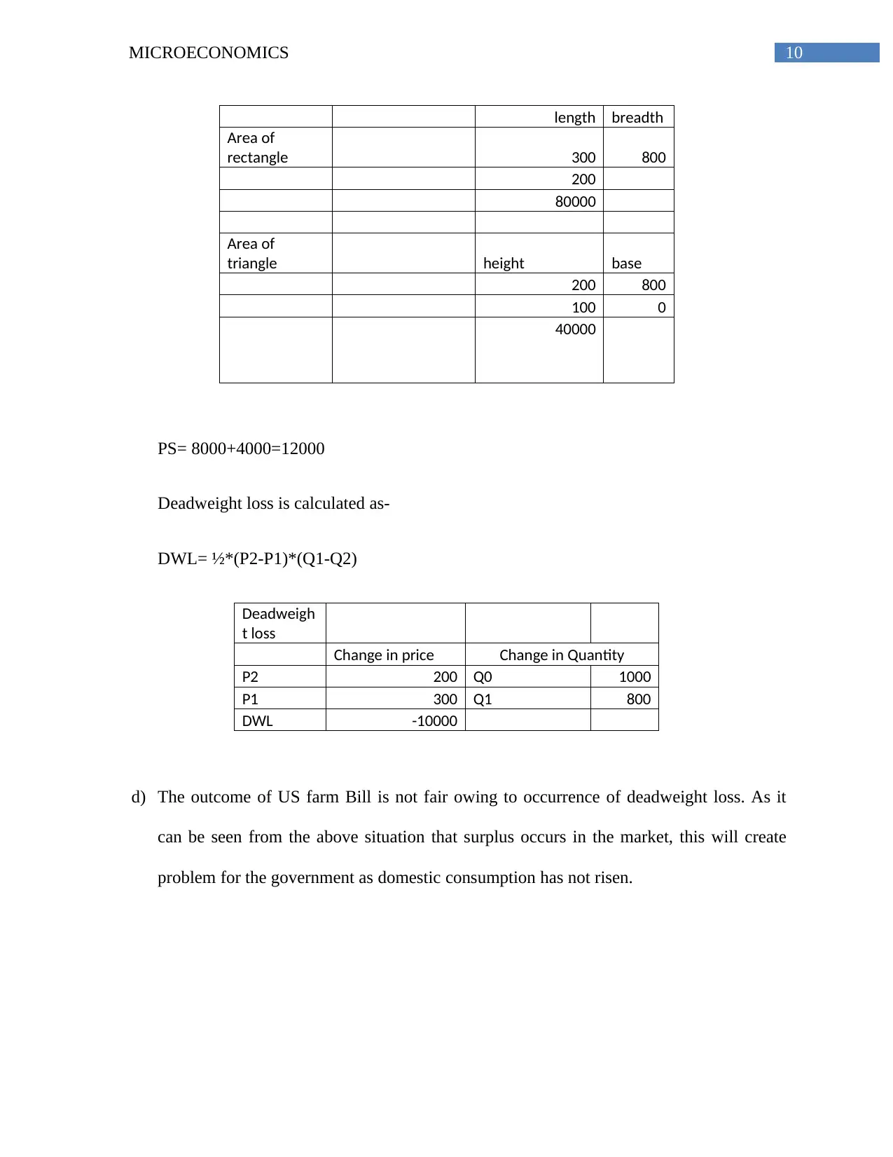
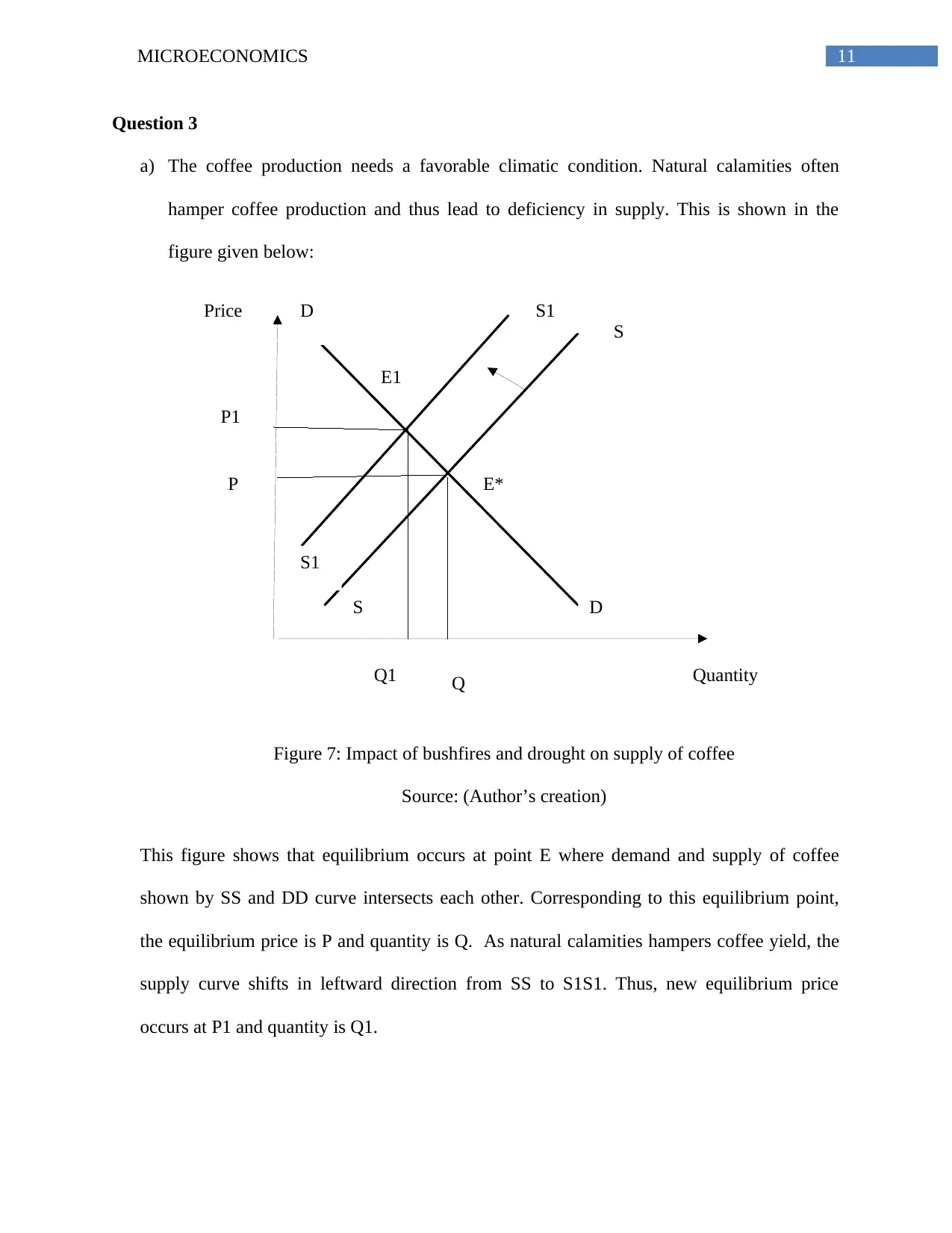
This microeconomics assignment analyzes several key concepts. It begins with an exploration of the Production Possibility Frontier (PPF), illustrating how it represents the maximum output combinations of two goods given limited resources. The assignment then delves into market equilibrium, using demand and supply functions to determine equilibrium price and quantity, and examines the effects of a government-imposed tax, including the calculation of deadweight loss and tax incidence. The analysis extends to the impact of the US Farm Bill on wheat prices and quantities, examining consumer and producer surplus, and deadweight loss. Finally, the assignment considers the coffee market, exploring how natural calamities and technological advancements affect supply, demand, and equilibrium prices, with case studies illustrating different scenarios of demand and supply shifts. The assignment uses diagrams and calculations to support its analysis.

Running head: MICROECONOMICS
MICROECONOMICS
Name of the Student
Name of the University
Author’s Note

1MICROECONOMICS
Table of Contents
Question1.........................................................................................................................................2
Question 2........................................................................................................................................4
Question 3......................................................................................................................................11
References......................................................................................................................................18

2MICROECONOMICS
Question1
a) Given the Newland’s production capacity, the PPF (Production Possibility Frontier)
for production of bicycles and cars are highlighted in the below diagram;
0 1000 2000 3000 4000 5000
0
5000
10000
15000
20000
25000
30000
35000
PPF
Cars
BICYCLES
CARS
A
B
Y
Table 1: Production Possibility Frontier of cars and bicycles
Source: (Author’s Creation)
b) The PPF curve mainly signifies maximum possible output of the two commodities
given the inputs such as resources. It generally assumes that all the inputs are
effectively utilized in production (Baumol & Blinder, 2015). Few variables involving
technology, laborers impact the resources and thereby it shows that point where PPF
lies. The PPF curve indicates two commodities production possibilities given the
fixed resources. Furthermore, this PPF curve helps to determine efficiency of
producing two goods at same time.
This diagram highlights PPF for the production of bicycles and cars. The point A as
well as point B on the curve signifies that resources are allocated efficiently by a

3MICROECONOMICS
particular economy. Point B indicates that if a country starts to manufacture large number
of bicycles, then they should divert those resources which are used for producing cars. On
the contrary, Point A highlights that if the nation starts to produce huge number of cars,
then they should give up some resources for manufacturing bicycles. Moving from the
point A to B, the economy will reduce total car production in comparison with rise in
total bicycle output. The point Y depicts that the resources are utilized inefficiently,
which indicates that the economy is not producing huge number of bicycle and cars even
though resources are given (Hall & Lieberman,, 2012).
The assumptions of the PPF are illustrated below:
 Technology that is to be utilized in production of goods is taken to be fixed
 It is assumed that resources are utilized efficiently
 The resources used for manufacturing commodities could be relocated in order to
manufacture another commodity(Taussig, 2013).
Properties of the PPF are explained below:
 The PPF curve is basically negatively sloped since variation in amount of one
commodity is indirectly related to variation in amount of another commodity
 The shape of PPF curve is mainly concave due to rise in marginal opportunity
cost.
c) The three major possibilities by which the Newland could meet rise in demand are
given below:
 This nation could increase supply of the two commodities in order to meet the
customer’s requirement.

4MICROECONOMICS
 Newland might bring in emerging technologies in order to meet increased demand
of the commodities.
 Import of commodities will facilitate Newland to meet the demand for these two
commodities, which in turn will increase its supply.
Question 2
Part 1
The demand for and supply of pizza function are given as under-
QD= 20-2P
Qs= P-1
The equilibrium in the market occurs when the demand curve cuts the supply curve, ie QD=Qs
20-2P=P-1
20+1=P+2P
21=3P
P=21/3=7
At P=7, QD=20-2*7=20-14=6, Qs= 7-1=6. The diagram is shown below:

5MICROECONOMICS
-5 0 5 10 15 20 25
0
2
4
6
8
10
12
MARKET EQUILIBRIUM
Qd
Qs
Output
Price
7
6
Figure 2: Market equilibrium before tax
Source: (as created by author)
Now if the government imposes $3 tax per pizza that is purchased, then the demand function will
be-
QD= 20-2(P+3)
Qs=P-1
The new market equilibrium is-
QD= Qs
20-2(P+3)=P-1
20-2P-6=P-1
3P=20-6+1

6MICROECONOMICS
3P=15
P=5
At P=5, Qd= 20-2(5+3)=20-16=4, Qs=5-1=4
-2 0 2 4 6 8 10 12 14 16
0
1
2
3
4
5
6
7
MARKET EQUILIBRIUM AFTER IMPOSITION OF TAX
Qd
Qs
Output
Price
4
Figure 3: Market equilibrium after tax
Source: (Author’s creation)
-5 0 5 10 15 20 25
0
2
4
6
8
10
12
MARKET EQUILIBRIUM
Qd
Qs
Output
Price
7
6
Deadweight by tax

7MICROECONOMICS
Figure 4: Deadweight loss generated by tax
Source: (Author’s creation)
Tax incidence portrays distribution of tax obligations that should be covered by both
seller as well as buyers (Sloman, Norris & Garrett, 2013). It reveals which buyers and producers
will give price of new tax. After imposition of tax, the new equilibrium price is now $7 per
pizza. This means that sellers pass the burden to purchasers, who will have to pay $1` more per
pizza. Meanwhile, while sellers will attain $2 less per pizza they sell.
Tax generates deadweight loss because it prevents the people from purchasing the
product that cost high after imposition of tax than it would be before imposition of tax.
Deadweight loss refers to loss of good economically which occurs owing to imposition of tax
(Taylor et al., 2014). The deadweight loss generated by tax –
Deadweight loss= ½*(P2-P1)*(Q1-Q2)= 3
Part 2
a)

8MICROECONOMICS
0 500 1000 1500 2000 2500
0
50
100
150
200
250
300
350
400
450
IMPACT IN MARKET EQUILIBRIUM
Quantity demanded
Quantity supplied
Quantity
Price
Figure 5: Impact of equilibrium quantity and price of wheat
Source: (Author’s creation)
The market equilibrium occurs when the demand and supply curve intersects each other
(Reisman, 2013). From the above diagram , it can be seen that the equilibrium price is $250 and
equilibrium quantity is 1000. The US Farm Bill indicates that domestic price of wheat is set at
$300, which is above the equilibrium point. As market price is set above the equilibrium price ,
the total quantity supplied becomes greater than total quantity demanded. This, it leads to
creation of surplus and hence equilibrium price of wheat will decline and equilibrium quantity
will increase.
b) The figure below reflects consumer surplus, producer surplus and deadweight loss. The
triangle abc is the consumer surplus and cbed is the producer surplus. The triangular section bfg
is the deadweight loss.

9MICROECONOMICS
0 500 1000 1500 2000 2500
0
50
100
150
200
250
300
350
400
450
CS, PS AND DEADWEIGHT LOSS
Quantity demanded
Quantity supplied
Quantity
Price
DW
L
cs
PS
bc
Figure 6: Consumer surplus, producer surplus and Deadweight loss
Source: (Author’s creation)
c) Consumer surplus relates to welfare measurement in which each person needs to attain
from consumption of commodity. It is calculated as –
CS= ½*(base*height)
Consume
r surplus
Qd Change in price
800 Pmax 400
0 Pd 300
CS 40000
Producer surplus is that excess amount which the producers obtain from selling of
products in market. It is estimated similar to that of consumer surplus.
Producer
surplus
a
d e
f
g

10MICROECONOMICS
length breadth
Area of
rectangle 300 800
200
80000
Area of
triangle height base
200 800
100 0
40000
PS= 8000+4000=12000
Deadweight loss is calculated as-
DWL= ½*(P2-P1)*(Q1-Q2)
Deadweigh
t loss
Change in price Change in Quantity
P2 200 Q0 1000
P1 300 Q1 800
DWL -10000
d) The outcome of US farm Bill is not fair owing to occurrence of deadweight loss. As it
can be seen from the above situation that surplus occurs in the market, this will create
problem for the government as domestic consumption has not risen.

11MICROECONOMICS
Quantity
Price
D
D
S
S
S1
S1
E*
E1
QQ1
P
P1
Question 3
a) The coffee production needs a favorable climatic condition. Natural calamities often
hamper coffee production and thus lead to deficiency in supply. This is shown in the
figure given below:
Figure 7: Impact of bushfires and drought on supply of coffee
Source: (Author’s creation)
This figure shows that equilibrium occurs at point E where demand and supply of coffee
shown by SS and DD curve intersects each other. Corresponding to this equilibrium point,
the equilibrium price is P and quantity is Q. As natural calamities hampers coffee yield, the
supply curve shifts in leftward direction from SS to S1S1. Thus, new equilibrium price
occurs at P1 and quantity is Q1.