Microgrid Design and Analysis Report: Electrical Power Systems
VerifiedAdded on 2023/04/20
|17
|4351
|242
Report
AI Summary
This report presents a detailed design and analysis of a microgrid system, focusing on integrating renewable energy sources like wind turbines and solar PV panels. It covers the modeling of key components, including wind turbines, PV modules, battery banks, and diesel generators. The report analyzes load demand, calculates power factors, and explores system optimization strategies to minimize operational costs and ensure reliable power delivery. The design incorporates a flowchart illustrating the operational strategy of the microgrid, along with tables and graphs that represent load demand characteristics and solar insolation data. The optimization process aims to economically dispatch power from different sources to meet consumer needs, considering the initial and operational costs of the system. The report concludes with an overview of the system's operation under various conditions, including scenarios where the microgrid relies on renewable sources, battery storage, and diesel generators to meet peak load demands.
Student
Instructor
Electrical Power System
Date
Instructor
Electrical Power System
Date
Paraphrase This Document
Need a fresh take? Get an instant paraphrase of this document with our AI Paraphraser
Microgrid design
1
Abstract
In order to curb atmospheric pollution which has been posing a menace to the existence of
ecological system, mainly caused by unbridled emission of hazardous gases and fumes, all
sectors of economy has a role to play. The possible solution in the energy sector has been
made possible by embracing green energy technology. This technology has numerous
advantages just to mention a few; they can be operated in a stand-alone mode, they can be set
anywhere on the planet with existence of driving forces (considerable wind and solar
insolation), and construction time is very minimal compared to other forms of energy
generation utility. This report has dealt with method of estimating capacity of prerequisite
components of microgrid for the given peal load and average load demand. It has also
explained load scheduling ford the different generation unities in analysis and flowchart
representation.
Introduction
A micro grid standalone system consists of the PV modules, wind turbine, diesel generators
and inverters and controllers, battery storage banks and panel controllers [1]. Wind power
energy is a form of green energy produced by conversion of kinetic energy of the wind into
electrical energy. Naturally, wind flows is caused by pressure difference caused by
heterogeneous solar radiation reaching earth’s atmospheric structures. To meet load
requirement of the grid based on the consumers’ need, the grid need to be supplied with
dispatchable electricity. Wind power is not dispatchable by the fact that it solely depends on
the natural characteristic of the wind. Therefore, the output power is not guaranteed to meet
consumers’ demand since the system is vulnerable to fluctuation patterns of wind speed.
Solar energy if very friendly to the environment since it is clean, soundless and does not emit
fumes into the atmosphere [2]. Electrical energy is generated by conversion solar energy from
sunlight into electrical energy using photovoltaic cells. Photons energy greater than
semiconductor’s band gap energy is absorbed when light strikes on the surface of the solar
cell ejecting electrons and creating numerous pair of electron-hole pair [8].
Modelling of wind power turbines.
The actual mechanical power of the rotor blades is extracted from the difference between
[3] upstream wind power and downstream wind power as shown in the equation below.
Pw= 1
2 (ρA V + V O
2 ) (V 2−V 2
O ) (1)
Where Pw power of the rotor, V ∧V oare upstream entrance and downstream exit wind
velocity.
Volumetric mass flow rate= ρA V +V O
2 (2)
Rearranging equation (1) algebraically;
Microgrid design
2
Pw= 1
2 ρA V 3
( 1+ V O
V ) [ 1− ( V O
V )
2
]
2
(3)
The above equation comprises of two fundamental concepts namely; the general wind power
formulae and the fraction of upstream wind.
Pw= 1
2 ρA V 3 CP (4)
Where CP the rotor’s power coefficient that is basically the fraction of the upstream wind
energy converted to mechanical energy and fed to electrical transducer.
Theoretically, for maximum power output of the wind power, CP is 0.59, which is greatly
defined by¿). This fraction is the function of Tip-speed Ratio (TSR) of the rotor.
For this design, horizontal-type rotor is highly recommended since it possesses higher TSR
compared to vertical-type rotor such as savonious and darrieus [3]. Location for the
installation of wind turbine should be characterized by continuous flow wind at a
considerable speed.. When the wind speed exceeds considered safe speed, known as cut-out
speed, that could pose damage risk to the rotor blades, braking system is triggered to bring
rotor to a standstill [4].
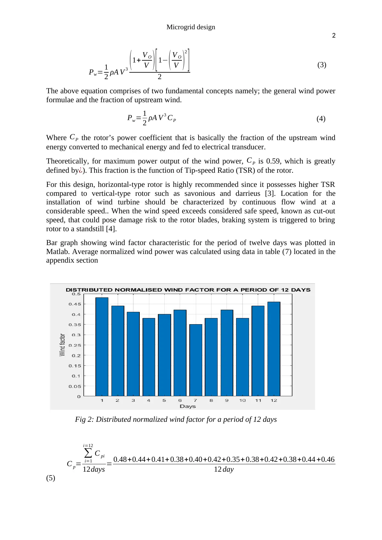
Bar graph showing wind factor characteristic for the period of twelve days was plotted in
Matlab. Average normalized wind power was calculated using data in table (7) located in the
appendix section
Fig 2: Distributed normalized wind factor for a period of 12 days
C p=
∑
i=1
i=12
C pi
12days = 0.48+0.44+ 0.41+ 0.38+0.40+0.42+0.35+ 0.38+0.42+0.38+0.44 +0.46
12 day
(5)
2
Pw= 1
2 ρA V 3
( 1+ V O
V ) [ 1− ( V O
V )
2
]
2
(3)
The above equation comprises of two fundamental concepts namely; the general wind power
formulae and the fraction of upstream wind.
Pw= 1
2 ρA V 3 CP (4)
Where CP the rotor’s power coefficient that is basically the fraction of the upstream wind
energy converted to mechanical energy and fed to electrical transducer.
Theoretically, for maximum power output of the wind power, CP is 0.59, which is greatly
defined by¿). This fraction is the function of Tip-speed Ratio (TSR) of the rotor.
For this design, horizontal-type rotor is highly recommended since it possesses higher TSR
compared to vertical-type rotor such as savonious and darrieus [3]. Location for the
installation of wind turbine should be characterized by continuous flow wind at a
considerable speed.. When the wind speed exceeds considered safe speed, known as cut-out
speed, that could pose damage risk to the rotor blades, braking system is triggered to bring
rotor to a standstill [4].
Bar graph showing wind factor characteristic for the period of twelve days was plotted in
Matlab. Average normalized wind power was calculated using data in table (7) located in the
appendix section
Fig 2: Distributed normalized wind factor for a period of 12 days
C p=
∑
i=1
i=12
C pi
12days = 0.48+0.44+ 0.41+ 0.38+0.40+0.42+0.35+ 0.38+0.42+0.38+0.44 +0.46
12 day
(5)
⊘ This is a preview!⊘
Do you want full access?
Subscribe today to unlock all pages.
Trusted by 1+ million students worldwide
Microgrid design
3
C p=0.413
Using data from table (3) in the appendix, and equation (5)
Pw= 1
2 ×1.225 kg /m3 ×31.9 m2 × ( 14 m
s )
3
×0.413 (6)
Pw=22142.72W
Mathematical modeling of the PV module.
The amount of electricity generated depends on factors such as the amount of solar
irradiance, type of the panels, and types of the inverters and converters used. Available power
(kWh) on the PV panel was calculated by the expression below.
PPV −out=PPV × Ƞpr × p . f × t (7)
Where Ƞpr is the performance ratio, p.f is the combined power factor, andt is the peak sun
hours. Number of panels required for the system can be estimated as;
N p= Average daily load demand
PPV −out
(8)
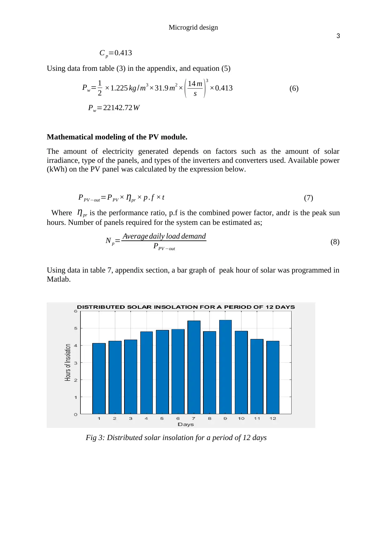
Using data in table 7, appendix section, a bar graph of peak hour of solar was programmed in
Matlab.
Fig 3: Distributed solar insolation for a period of 12 days
3
C p=0.413
Using data from table (3) in the appendix, and equation (5)
Pw= 1
2 ×1.225 kg /m3 ×31.9 m2 × ( 14 m
s )
3
×0.413 (6)
Pw=22142.72W
Mathematical modeling of the PV module.
The amount of electricity generated depends on factors such as the amount of solar
irradiance, type of the panels, and types of the inverters and converters used. Available power
(kWh) on the PV panel was calculated by the expression below.
PPV −out=PPV × Ƞpr × p . f × t (7)
Where Ƞpr is the performance ratio, p.f is the combined power factor, andt is the peak sun
hours. Number of panels required for the system can be estimated as;
N p= Average daily load demand
PPV −out
(8)
Using data in table 7, appendix section, a bar graph of peak hour of solar was programmed in
Matlab.
Fig 3: Distributed solar insolation for a period of 12 days
Paraphrase This Document
Need a fresh take? Get an instant paraphrase of this document with our AI Paraphraser
Microgrid design
4
t=
∑
i=1
12
Hrs
12 = 4.12+4.25+4.32+4.78+ 4.88+ 4.92+ 5.41+ 4.81+5.47+4.82+ 4.35+4.25
12
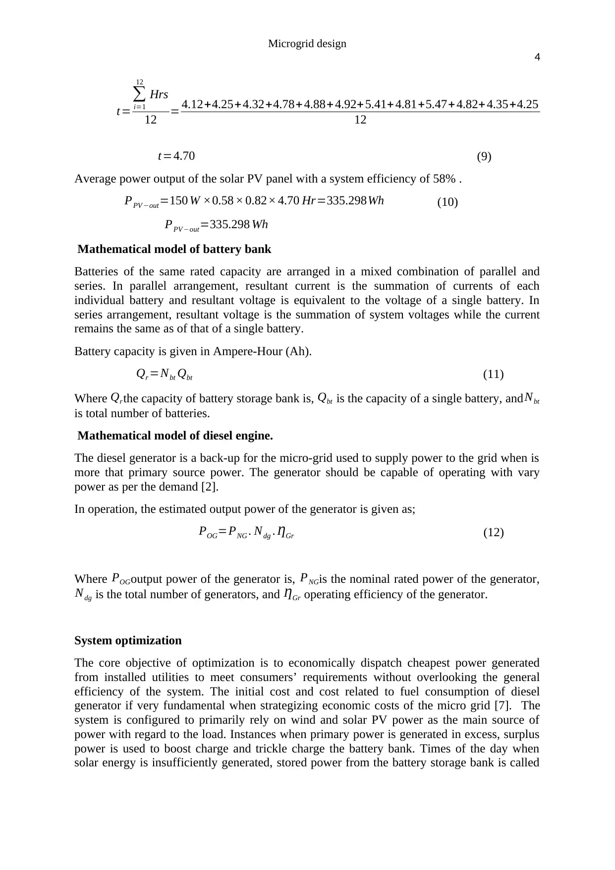
t=4.70 (9)
Average power output of the solar PV panel with a system efficiency of 58% .
PPV −out=150 W ×0.58 × 0.82× 4.70 Hr=335.298Wh (10)
PPV −out=335.298 Wh
Mathematical model of battery bank
Batteries of the same rated capacity are arranged in a mixed combination of parallel and
series. In parallel arrangement, resultant current is the summation of currents of each
individual battery and resultant voltage is equivalent to the voltage of a single battery. In
series arrangement, resultant voltage is the summation of system voltages while the current
remains the same as of that of a single battery.
Battery capacity is given in Ampere-Hour (Ah).
Qr =Nbt Qbt (11)
Where Qrthe capacity of battery storage bank is, Qbt is the capacity of a single battery, and Nbt
is total number of batteries.
Mathematical model of diesel engine.
The diesel generator is a back-up for the micro-grid used to supply power to the grid when is
more that primary source power. The generator should be capable of operating with vary
power as per the demand [2].
In operation, the estimated output power of the generator is given as;
POG=PNG . Ndg . ȠGr (12)
Where POGoutput power of the generator is, PNGis the nominal rated power of the generator,
Ndg is the total number of generators, and ȠGr operating efficiency of the generator.
System optimization
The core objective of optimization is to economically dispatch cheapest power generated
from installed utilities to meet consumers’ requirements without overlooking the general
efficiency of the system. The initial cost and cost related to fuel consumption of diesel
generator if very fundamental when strategizing economic costs of the micro grid [7]. The
system is configured to primarily rely on wind and solar PV power as the main source of
power with regard to the load. Instances when primary power is generated in excess, surplus
power is used to boost charge and trickle charge the battery bank. Times of the day when
solar energy is insufficiently generated, stored power from the battery storage bank is called
4
t=
∑
i=1
12
Hrs
12 = 4.12+4.25+4.32+4.78+ 4.88+ 4.92+ 5.41+ 4.81+5.47+4.82+ 4.35+4.25
12
t=4.70 (9)
Average power output of the solar PV panel with a system efficiency of 58% .
PPV −out=150 W ×0.58 × 0.82× 4.70 Hr=335.298Wh (10)
PPV −out=335.298 Wh
Mathematical model of battery bank
Batteries of the same rated capacity are arranged in a mixed combination of parallel and
series. In parallel arrangement, resultant current is the summation of currents of each
individual battery and resultant voltage is equivalent to the voltage of a single battery. In
series arrangement, resultant voltage is the summation of system voltages while the current
remains the same as of that of a single battery.
Battery capacity is given in Ampere-Hour (Ah).
Qr =Nbt Qbt (11)
Where Qrthe capacity of battery storage bank is, Qbt is the capacity of a single battery, and Nbt
is total number of batteries.
Mathematical model of diesel engine.
The diesel generator is a back-up for the micro-grid used to supply power to the grid when is
more that primary source power. The generator should be capable of operating with vary
power as per the demand [2].
In operation, the estimated output power of the generator is given as;
POG=PNG . Ndg . ȠGr (12)
Where POGoutput power of the generator is, PNGis the nominal rated power of the generator,
Ndg is the total number of generators, and ȠGr operating efficiency of the generator.
System optimization
The core objective of optimization is to economically dispatch cheapest power generated
from installed utilities to meet consumers’ requirements without overlooking the general
efficiency of the system. The initial cost and cost related to fuel consumption of diesel
generator if very fundamental when strategizing economic costs of the micro grid [7]. The
system is configured to primarily rely on wind and solar PV power as the main source of
power with regard to the load. Instances when primary power is generated in excess, surplus
power is used to boost charge and trickle charge the battery bank. Times of the day when
solar energy is insufficiently generated, stored power from the battery storage bank is called
Microgrid design
5
upon to compensate for the deficit in conjunction with the wind power. At this moment,
diesel generators are still not in operation.
At peak load demand, primary power combined with battery storage bank probably wouldn’t
be able to service consumers. It is at this moment when diesel generators come into the mix
to supplement the power deficit. However, the diesel engines are not expected to run in full
load condition unless otherwise so as to minimize the fuel price. In other words, power
tapped from the diesel generators should be enough to mitigate against the flaw created.
Optimizing expressions dealt with majorly strives to minimize the fuel cost which is the
most expensive as far as operation cost is concerned. The initial cost of establishing the
system covers purchase costs of diesel generators, a complete system of solar PV, wind
turbines system, and storage bank system and labor.
Cost of transmitting power can be explained by the time-function expression below.
Coperation=δt n ∑
t =1
T
Cd ( t )+∑
f =1
n
Ci (13)
Where Cd ( t ) ( C=182,000 $ / MVA/ km )is the cost of fuel at δ t operating time of the diesel
engine,n is number of engaged generators, and Ci is the cost incurred due to power loss
along the length of feeder lines . Operation the micro-grid at a given time is given by the
equations below.
Power to the grid;
Ppv ( t ) +Pw ( t ) + Pbat ( t ) + PG ( t ) =PL ( t ) (14)
State of charge (SoC) of the battery storage bank
SoCmin ≤ SoC(t ) ≤ SoCmax (15)
Charge-discharge condition of the battery storage bank
1 ≤ Bdischarge ( t ) +Bcharge ( t ) ≥1 (16)
Where Ppv ( t ) is total PV solar power, Pw ( t ) is total wind power, PG ( t ) is total generator
power, Pbat ( t ) is stored power and PL ( t ) is the load demand. For optimum operation and
economic dispatch, constrains were introduced the expression in equation (21).
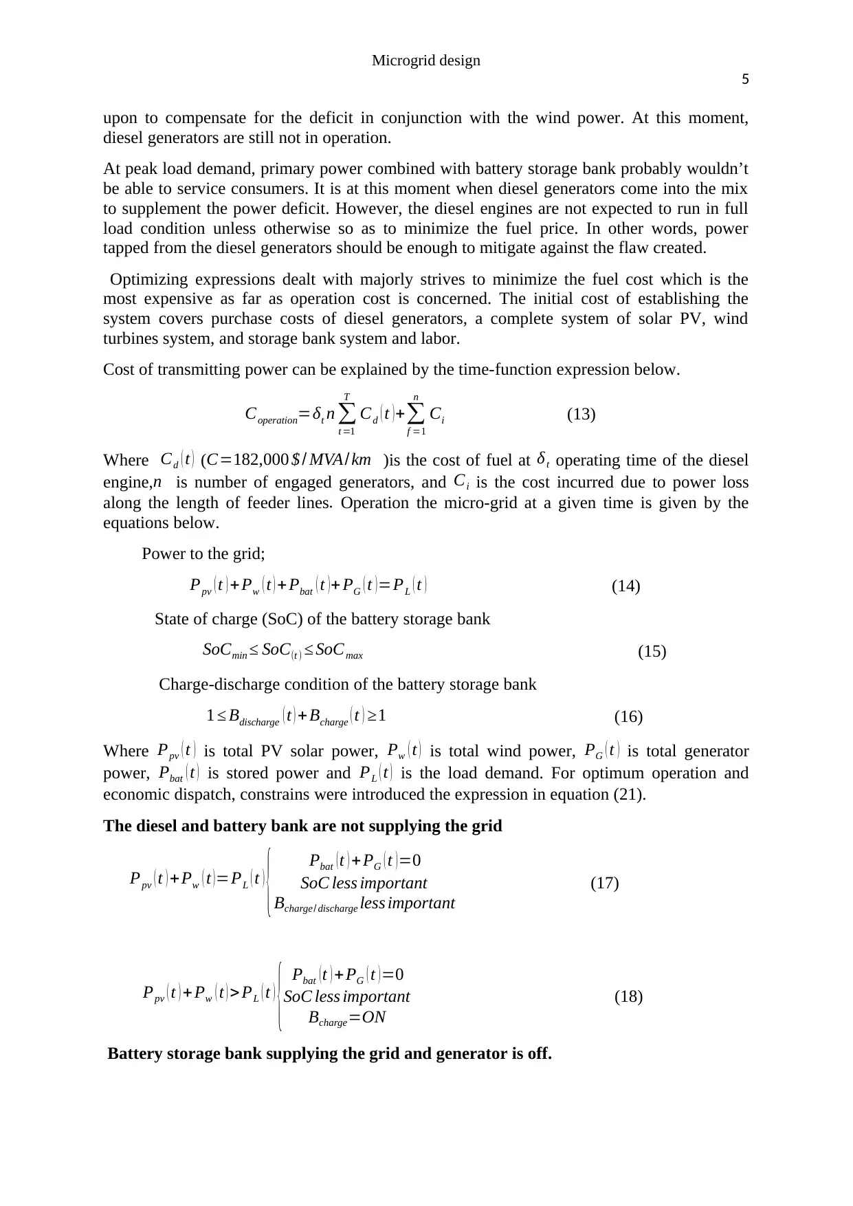
The diesel and battery bank are not supplying the grid
Ppv ( t ) + Pw ( t )=PL ( t )
{ Pbat (t ) +PG ( t )=0
SoC less important
Bcharge/ discharge less important
(17)
Ppv ( t ) + Pw ( t ) > PL ( t )
{ Pbat (t ) + PG ( t )=0
SoC less important
Bcharge=ON
(18)
Battery storage bank supplying the grid and generator is off.
5
upon to compensate for the deficit in conjunction with the wind power. At this moment,
diesel generators are still not in operation.
At peak load demand, primary power combined with battery storage bank probably wouldn’t
be able to service consumers. It is at this moment when diesel generators come into the mix
to supplement the power deficit. However, the diesel engines are not expected to run in full
load condition unless otherwise so as to minimize the fuel price. In other words, power
tapped from the diesel generators should be enough to mitigate against the flaw created.
Optimizing expressions dealt with majorly strives to minimize the fuel cost which is the
most expensive as far as operation cost is concerned. The initial cost of establishing the
system covers purchase costs of diesel generators, a complete system of solar PV, wind
turbines system, and storage bank system and labor.
Cost of transmitting power can be explained by the time-function expression below.
Coperation=δt n ∑
t =1
T
Cd ( t )+∑
f =1
n
Ci (13)
Where Cd ( t ) ( C=182,000 $ / MVA/ km )is the cost of fuel at δ t operating time of the diesel
engine,n is number of engaged generators, and Ci is the cost incurred due to power loss
along the length of feeder lines . Operation the micro-grid at a given time is given by the
equations below.
Power to the grid;
Ppv ( t ) +Pw ( t ) + Pbat ( t ) + PG ( t ) =PL ( t ) (14)
State of charge (SoC) of the battery storage bank
SoCmin ≤ SoC(t ) ≤ SoCmax (15)
Charge-discharge condition of the battery storage bank
1 ≤ Bdischarge ( t ) +Bcharge ( t ) ≥1 (16)
Where Ppv ( t ) is total PV solar power, Pw ( t ) is total wind power, PG ( t ) is total generator
power, Pbat ( t ) is stored power and PL ( t ) is the load demand. For optimum operation and
economic dispatch, constrains were introduced the expression in equation (21).
The diesel and battery bank are not supplying the grid
Ppv ( t ) + Pw ( t )=PL ( t )
{ Pbat (t ) +PG ( t )=0
SoC less important
Bcharge/ discharge less important
(17)
Ppv ( t ) + Pw ( t ) > PL ( t )
{ Pbat (t ) + PG ( t )=0
SoC less important
Bcharge=ON
(18)
Battery storage bank supplying the grid and generator is off.
⊘ This is a preview!⊘
Do you want full access?
Subscribe today to unlock all pages.
Trusted by 1+ million students worldwide
Microgrid design
6
Ppv ( t ) + Pw ( t ) + Pbat ( t ) =PL ( t )
{ PG ( t ) =0
SoCmin< SoC(t) ≤ SoCmax
Bcharge=OFF
(19)
Battery bank and generator supplying the grid
Ppv ( t ) + Pw ( t ) + Pbat ( t )+ PG ( t )=PL ( t )
{Ppv ( t )+ Pw ( t ) +Pbat ( t ) <PL ( t )
SoCmin<SoC(t )≤ SoCmax
Bcharge=OFF
(20)
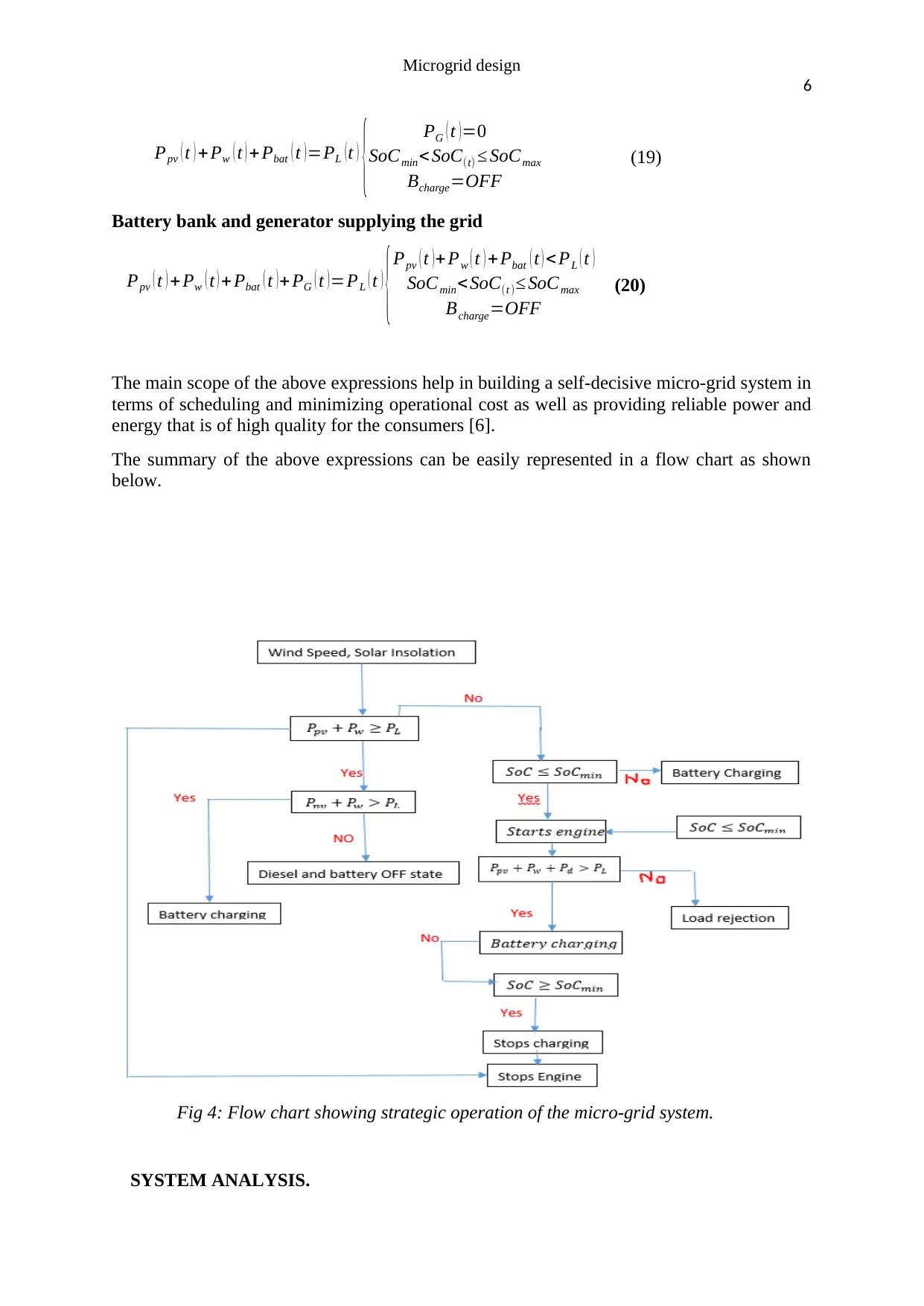
The main scope of the above expressions help in building a self-decisive micro-grid system in
terms of scheduling and minimizing operational cost as well as providing reliable power and
energy that is of high quality for the consumers [6].
The summary of the above expressions can be easily represented in a flow chart as shown
below.
Fig 4: Flow chart showing strategic operation of the micro-grid system.
SYSTEM ANALYSIS.
6
Ppv ( t ) + Pw ( t ) + Pbat ( t ) =PL ( t )
{ PG ( t ) =0
SoCmin< SoC(t) ≤ SoCmax
Bcharge=OFF
(19)
Battery bank and generator supplying the grid
Ppv ( t ) + Pw ( t ) + Pbat ( t )+ PG ( t )=PL ( t )
{Ppv ( t )+ Pw ( t ) +Pbat ( t ) <PL ( t )
SoCmin<SoC(t )≤ SoCmax
Bcharge=OFF
(20)
The main scope of the above expressions help in building a self-decisive micro-grid system in
terms of scheduling and minimizing operational cost as well as providing reliable power and
energy that is of high quality for the consumers [6].
The summary of the above expressions can be easily represented in a flow chart as shown
below.
Fig 4: Flow chart showing strategic operation of the micro-grid system.
SYSTEM ANALYSIS.
Paraphrase This Document
Need a fresh take? Get an instant paraphrase of this document with our AI Paraphraser
Microgrid design
7
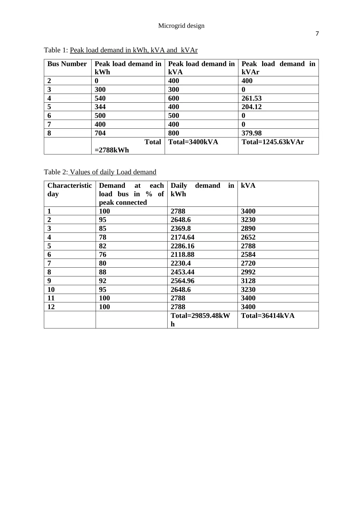
Table 1: Peak load demand in kWh, kVA and kVAr
Bus Number Peak load demand in
kWh
Peak load demand in
kVA
Peak load demand in
kVAr
2 0 400 400
3 300 300 0
4 540 600 261.53
5 344 400 204.12
6 500 500 0
7 400 400 0
8 704 800 379.98
Total
=2788kWh
Total=3400kVA Total=1245.63kVAr
Table 2: Values of daily Load demand
Characteristic
day
Demand at each
load bus in % of
peak connected
Daily demand in
kWh
kVA
1 100 2788 3400
2 95 2648.6 3230
3 85 2369.8 2890
4 78 2174.64 2652
5 82 2286.16 2788
6 76 2118.88 2584
7 80 2230.4 2720
8 88 2453.44 2992
9 92 2564.96 3128
10 95 2648.6 3230
11 100 2788 3400
12 100 2788 3400
Total=29859.48kW
h
Total=36414kVA
7
Table 1: Peak load demand in kWh, kVA and kVAr
Bus Number Peak load demand in
kWh
Peak load demand in
kVA
Peak load demand in
kVAr
2 0 400 400
3 300 300 0
4 540 600 261.53
5 344 400 204.12
6 500 500 0
7 400 400 0
8 704 800 379.98
Total
=2788kWh
Total=3400kVA Total=1245.63kVAr
Table 2: Values of daily Load demand
Characteristic
day
Demand at each
load bus in % of
peak connected
Daily demand in
kWh
kVA
1 100 2788 3400
2 95 2648.6 3230
3 85 2369.8 2890
4 78 2174.64 2652
5 82 2286.16 2788
6 76 2118.88 2584
7 80 2230.4 2720
8 88 2453.44 2992
9 92 2564.96 3128
10 95 2648.6 3230
11 100 2788 3400
12 100 2788 3400
Total=29859.48kW
h
Total=36414kVA
Microgrid design
8
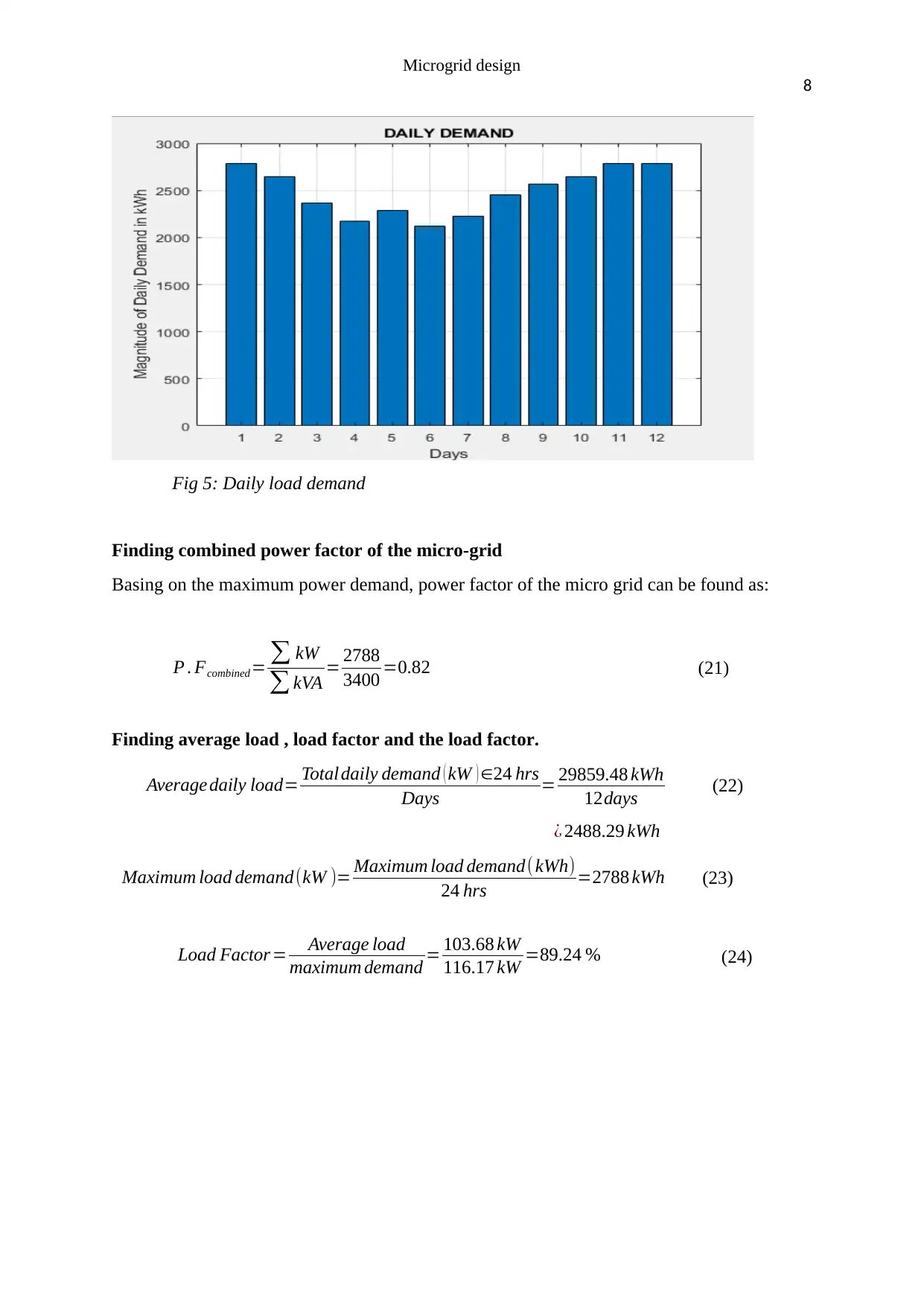
Fig 5: Daily load demand
Finding combined power factor of the micro-grid
Basing on the maximum power demand, power factor of the micro grid can be found as:
P . Fcombined= ∑ kW
∑ kVA = 2788
3400 =0.82 (21)
Finding average load , load factor and the load factor.
Average daily load= Total daily demand ( kW ) ∈24 hrs
Days = 29859.48 kWh
12days (22)
¿ 2488.29 kWh
Maximum load demand(kW )= Maximum load demand( kWh)
24 hrs =2788 kWh (23)
Load Factor= Average load
maximum demand = 103.68 kW
116.17 kW =89.24 % (24)
8
Fig 5: Daily load demand
Finding combined power factor of the micro-grid
Basing on the maximum power demand, power factor of the micro grid can be found as:
P . Fcombined= ∑ kW
∑ kVA = 2788
3400 =0.82 (21)
Finding average load , load factor and the load factor.
Average daily load= Total daily demand ( kW ) ∈24 hrs
Days = 29859.48 kWh
12days (22)
¿ 2488.29 kWh
Maximum load demand(kW )= Maximum load demand( kWh)
24 hrs =2788 kWh (23)
Load Factor= Average load
maximum demand = 103.68 kW
116.17 kW =89.24 % (24)
⊘ This is a preview!⊘
Do you want full access?
Subscribe today to unlock all pages.
Trusted by 1+ million students worldwide
Microgrid design
9
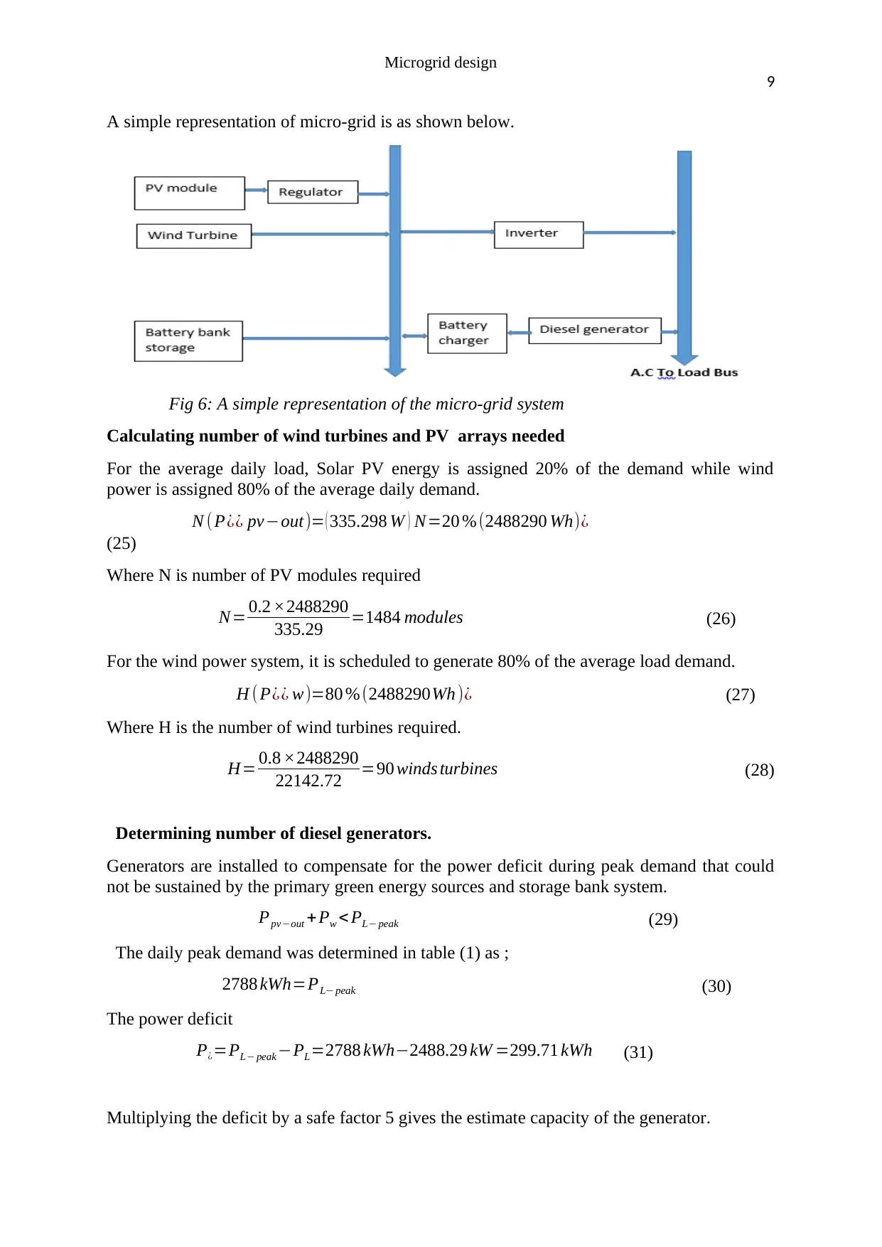
A simple representation of micro-grid is as shown below.
Fig 6: A simple representation of the micro-grid system
Calculating number of wind turbines and PV arrays needed
For the average daily load, Solar PV energy is assigned 20% of the demand while wind
power is assigned 80% of the average daily demand.
N ( P¿¿ pv−out)= ( 335.298 W ) N=20 % (2488290 Wh)¿
(25)
Where N is number of PV modules required
N= 0.2 ×2488290
335.29 =1484 modules (26)
For the wind power system, it is scheduled to generate 80% of the average load demand.
H ( P¿¿ w)=80 % (2488290Wh )¿ (27)
Where H is the number of wind turbines required.
H= 0.8 ×2488290
22142.72 =90 winds turbines (28)
Determining number of diesel generators.
Generators are installed to compensate for the power deficit during peak demand that could
not be sustained by the primary green energy sources and storage bank system.
Ppv−out +Pw < PL− peak (29)
The daily peak demand was determined in table (1) as ;
2788 kWh=PL− peak (30)
The power deficit
P¿=PL− peak −PL=2788 kWh−2488.29 kW =299.71 kWh (31)
Multiplying the deficit by a safe factor 5 gives the estimate capacity of the generator.
9
A simple representation of micro-grid is as shown below.
Fig 6: A simple representation of the micro-grid system
Calculating number of wind turbines and PV arrays needed
For the average daily load, Solar PV energy is assigned 20% of the demand while wind
power is assigned 80% of the average daily demand.
N ( P¿¿ pv−out)= ( 335.298 W ) N=20 % (2488290 Wh)¿
(25)
Where N is number of PV modules required
N= 0.2 ×2488290
335.29 =1484 modules (26)
For the wind power system, it is scheduled to generate 80% of the average load demand.
H ( P¿¿ w)=80 % (2488290Wh )¿ (27)
Where H is the number of wind turbines required.
H= 0.8 ×2488290
22142.72 =90 winds turbines (28)
Determining number of diesel generators.
Generators are installed to compensate for the power deficit during peak demand that could
not be sustained by the primary green energy sources and storage bank system.
Ppv−out +Pw < PL− peak (29)
The daily peak demand was determined in table (1) as ;
2788 kWh=PL− peak (30)
The power deficit
P¿=PL− peak −PL=2788 kWh−2488.29 kW =299.71 kWh (31)
Multiplying the deficit by a safe factor 5 gives the estimate capacity of the generator.
Paraphrase This Document
Need a fresh take? Get an instant paraphrase of this document with our AI Paraphraser
Microgrid design
10
NPg =5 P¿=1500 kWh (32)
The generator equation modelled and the power rating retrieved from table (6) in the
appendix
POG=Pg . N dg . ȠGr =¿ 1000kW.Ndg ×0.82 (33)
Ndg= 1500 kWh
1000 kWh× 0.82 =18Generators (34)
Generators are installed near load centers with high peak demand.
Capacity of feeders.
Feeder(34)
The total load at bus 4 is given by
Loadbus4 =Load+ Lossbranch 4=Load +2 %Load (35)
Loadbus4 =600 kVA + 0.02(600)kVA =612 kVA
Assuming voltage at the bus is maintained at 415 V, feeder current is obtained as
I f 34= Loadbus4
√3 × 415V = 612000
√ 3× 415 V =851.41 A (36)
Finding IR loss of the feeder.
IRloss =851.41 A × ( 0.3 km × 0.08 Ω/km ) =20.43 VA (37)
The capacity of feeder (34) thereof is obtained using the equation below
Total load (Sf 34 )=Loadbus 4 + IR (38)
Sf 34= ( 612+0.02043 ) kVA ¿ 612.02043 kVA
Feeder (35)
The total load at bus 5 is determined by the equation below
Loadbus5=Load + Lossbranch5=Loadbus5 =Load+2 %Load (39)
Loadbus.5 .=400 kVA+0.02(400)kVA =408 kVA
Assuming voltage at the bus is maintained at 415 V, feeder current is obtained as
I f 35= Loadbus5
√3× 415 V = 408000
√3 × 415 V =567.6118 A (40)
Finding IR loss of the feeder.
IRloss =567.6118 A × ( 0.2 km× 0.08 Ω/km )=9.082 VA (41)
The capacity of feeder (35) thereof is obtained using the equation below
Sf 35=Loadbus5 + IR= ( 408+0.009082 ) kVA=408.009082 kVA (42)
Feeder (68)
Microgrid design
11
Total load =Loadbus8 + Lossbranch 8 (43)
The total load at bus 8 is given by
Loadbus8 =Load+Lossbranch8=800 kVA +0.02 ( 800 ) kVA=816 kVA (44)
Assuming voltage at the bus is maintained at 415 V, feeder current is obtained as
I f 68= Loadbus8
√3× 415 V = 816000VA
√ 3× 415 V =1135.224 A (45)
Finding IR loss of feeder (68).
IRloss =1135.224 A × ( 0.3 km ×0.08 Ω /km ) =27.245VA (46)
The capacity of feeder (68) thereof is obtained using the equation below
Sf 68=Loadbus4 +IR=( 816+ 0.027245 ) kVA=816.027245 kVA (47)
Feeder (67)
The total load at bus 7 is given by
Loadbus7 =Load+ Lossbranch7=400 kVA +0.02( 400) kVA=408 kVA (48)
Assuming voltage at the bus is maintained at 240 V, feeder current is obtained as
I f 67= Loadbus7
240 V = 408000
240 V =1700 A (49)
Finding IR loss of the feeder.
IRloss =1700 A × ( 0.2 km× 0.08 Ω/km )=27.2 VA (50)
The capacity of feeder (67) thereof is obtained using the equation below
Sf 67=Loadbus7 + IR= ( 408+ 0.0272 ) kVA=408.0272kVA (60)
Feeder (23)
Loadbus3=Sf 35 +Sf 34+Branch3 (61)
Loadbus3=408.009082+612.02043+ ( 300+0.02 ×300 ) kVA =1326.0295 kVA
Calculating current at branch (3) supplied with single phase.
Ibranch3= ( 300+0.02 ×300 ) kVA
240V =1275 A (62)
Total current in feeder (23) is determined by
I f 23=Ibranch3 + I f 35 +I f 34=1275 A+851.41 A+567.61 A=2694.02 A (63)
Finding IR losses in feeder (23)
Lossf 23=I f 23 (1.2 km× 0.08 Ω/km)=2694.02(1.2 km× 0.08 Ω/km) (64)
⊘ This is a preview!⊘
Do you want full access?
Subscribe today to unlock all pages.
Trusted by 1+ million students worldwide
1 out of 17

Your All-in-One AI-Powered Toolkit for Academic Success.
+13062052269
info@desklib.com
Available 24*7 on WhatsApp / Email
![[object Object]](/_next/static/media/star-bottom.7253800d.svg)
Unlock your academic potential
Copyright © 2020–2026 A2Z Services. All Rights Reserved. Developed and managed by ZUCOL.