Math 3001 Assignment 2: In-Depth Investigation of Two Functions

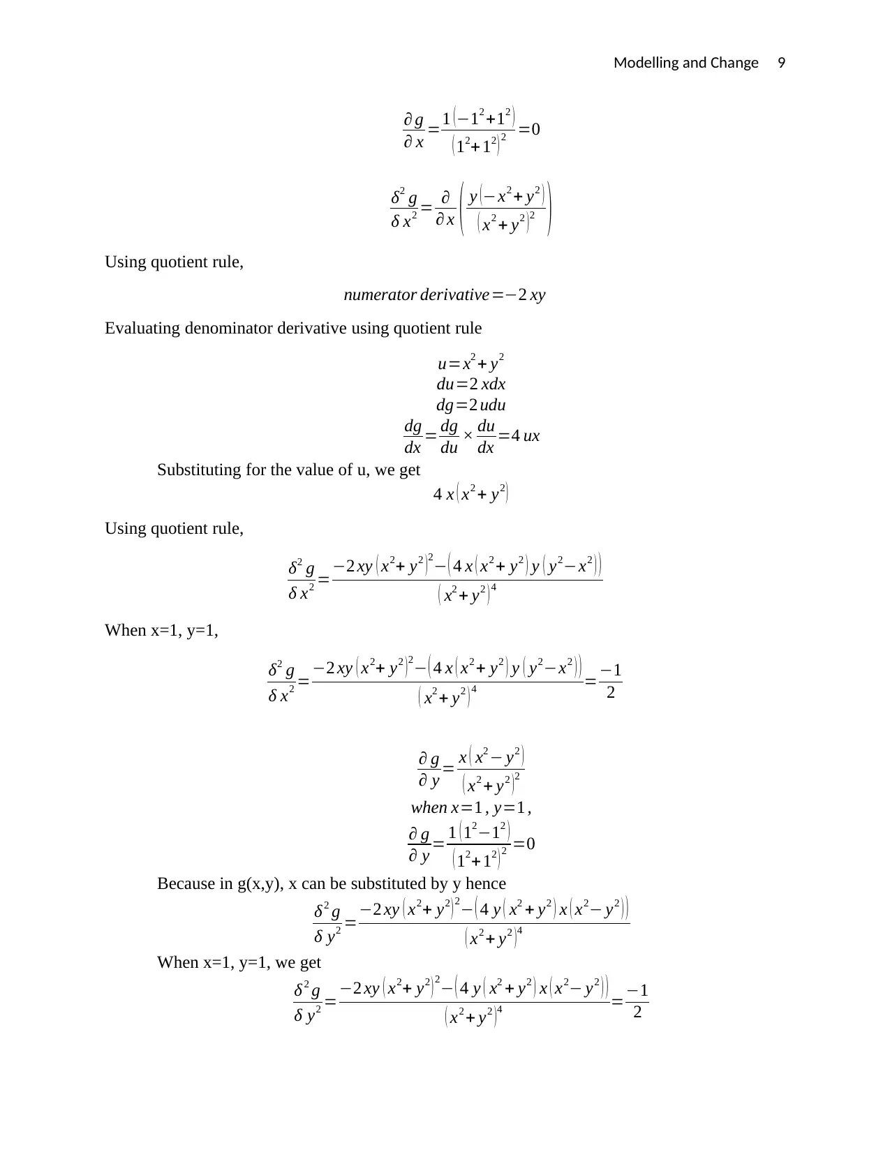
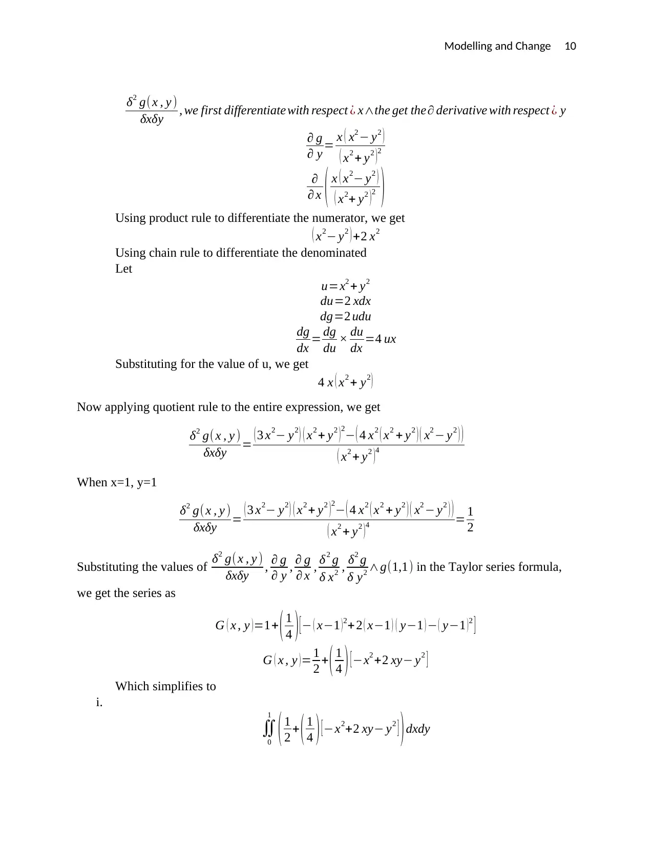
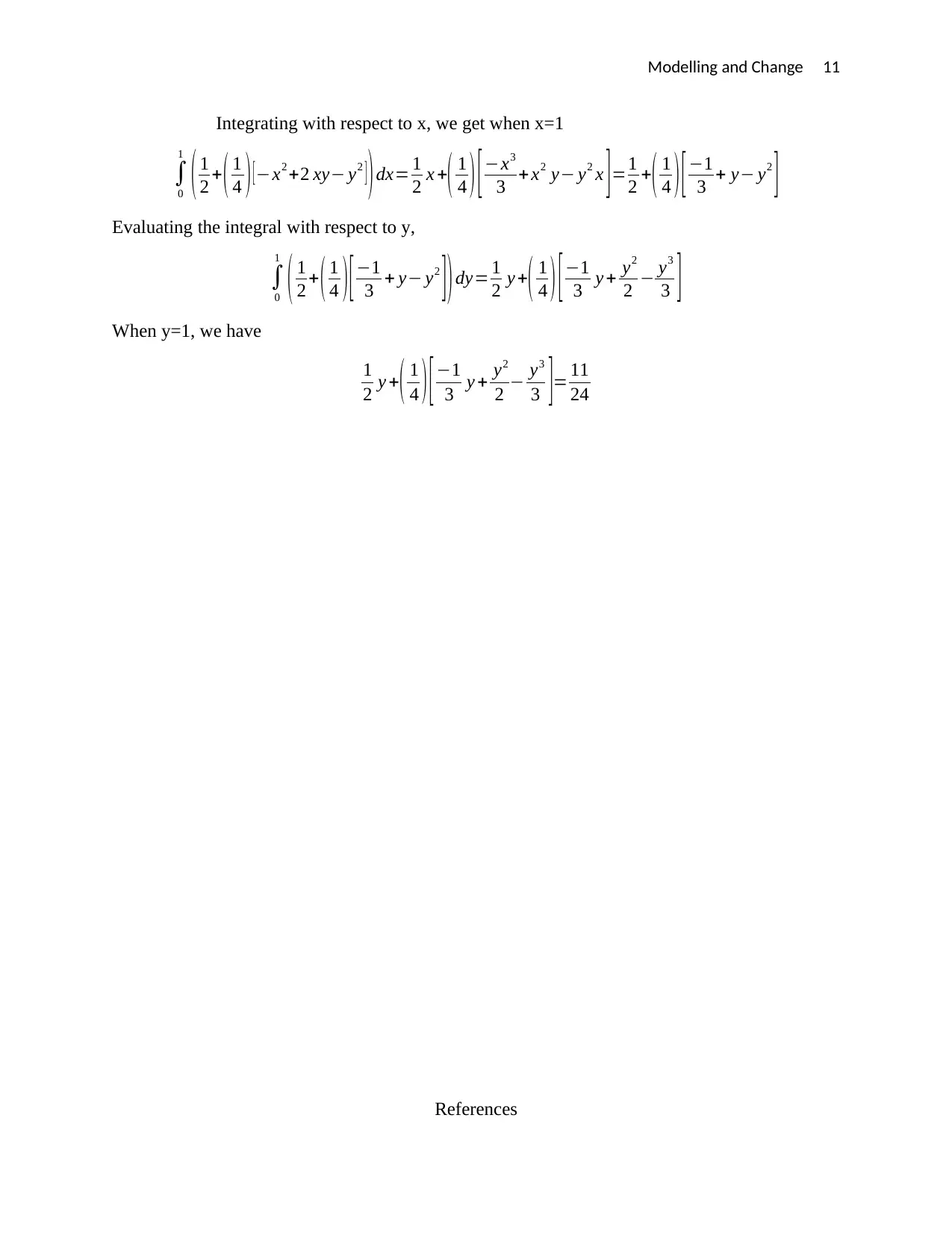
This assignment solution for Math 3001, "Modelling and Change (Advanced Level)", delves into the in-depth investigation of two functions: f(x) = sin^2(x) and g(x, y) = x^2 - xy + y^2. Part 1 explores the use of tangent lines, planes, and Taylor polynomials for approximate integration, analyzing the areas and volumes derived from these methods. It contrasts the accuracy of polynomial approximations for single and two-variable functions, presenting numerical values and equations for tangent lines and planes. Part 2 focuses on calculating derivatives using the chain, quotient, and product rules. The solution provides detailed steps for evaluating derivatives, finding equations for tangent lines, and constructing Taylor series approximations. The assignment concludes with references to relevant calculus and advanced mathematics resources.

Modelling and Change 1
Math 3001: Modelling and Change (Advanced Level), Assignment 2: In-Depth Investigation of
two functions
Course Number ………………………………………………………………….
Name …………………………………………………………………………………..
Name of group members………………………………………………………………

Modelling and Change 2
Part 1
a. Purpose of the presentation.
To explore the use of tangent lines, tangent planes and Taylor polynomials for
approximate integration.
b.
c. Equation of the tangent line
The gradient of the tangent line
f ' ( x)=sin 2 x
Equation of the tangent line at x= π
2
f ( x ) =1
d. area under f(x) between x = 0 and x = π
=π/2 square units
area under the tangent line at x = π/ 2
π/ 2
The two areas are similar
The area under the curve is greater than the area under the tangent line at x = π/ 2
e. Importance of the area under the tangent line
This area provides a linear approximation of the area under the curve. It reveals
information on the areas that is covered by the function if we use a line that passes
through the point only once
f.
T 2=x2

Modelling and Change 3
T 3=0
g.
Blue-the tangent line of f(x) at x=pi/2
Red= f(x)
h.
∫
0
π
T 2=¿ 10.33542 ¿
∫
0
π
T 3=0
i. The use of Polynomial approximation of a single variable function is poor method of
approximating integration of single-variable function in this case because the areas using
using this method is way larger than the actual area.
j.

Modelling and Change 4
k. g ( x , y )= xy
x2+ y2
Volume=∬ xy
x2+ y2 dR=0.34657 cubic units
l. At point (1,1), the equation of a plane that is tangential to g(x,y)=
f ( x , y )=1
m. volume between the tangent plane and xy-plane, for R = [0, 1] × [0, 1].
1 cubic units
n. The volume under the tangent plane reveals a linear approximation of the volume being
evaluated.
o. Equation of the second-degree Taylor polynomial G(x, y) of g(x, y) at the point (1, 1).
G ( x , y )= 1
2 + ( 1
4 ) [−x2 +2 xy− y2 ]
p.
q. Present the numerical value of the double integral
=11/24
r. we know that the level curve g(x, y) = 0 exists is known to exist because for the
coordinates x=0,y=0, g(x,y)=0

Modelling and Change 5
s. Since g(x,y)=0 exist, it implies that the function gets larger in every direction. The
higher order derivatives will get more and more insignificant thus improving Taylor
approximation.
t. use of polynomial approximations of two-variable functions as a method of
approximating integration of two-variable functions is relatively more accurate compared
to the same concept for a single variable function based on the results. This because the
actual integration yields 0.34657 while Taylor approximation yields 11/24 for 2-variable
which compares closer now that only two terms were used. The accuracy would have
been improved by using more terms in Taylor approximation.

Modelling and Change 6
Part 2.
a.
f ( x )=sin2 x
The derivative
f ' ( x )= d
dx ( sin2 x )
From chain rule, we let u=sinx, du=cosx.dx
Hence we have
¿ d
du ( u2 ) d
dx ( sin ( x ) )=2ucos ( x )
substituting u=sin (x )
2 ¿
When x= π
2 , f '
( π
2 )=0
y−1=0 ¿
y=1
b.
∫
0
π
sin2 xdx
¿ trigonometric identities sin2 xdx= 1−cos 2 x
2
∫
0
π
sin2 xdx=∫
0
π
1−cos 2 x
2 dx=¿ π
2 =1.57079 ¿
Area under tangent line
1 × π
2 = π
2
c.
f ( x ) P ( x )=∑
0
n f k (a)
k ! xk
We therefore evaluate the derivatives as follows
f 1 ( x )= ( f 0 ( x ) )'
= ( sin2 x )'
=sin (2 x )
f 2 ( x ) = ( f 1 ( x ) ) '
= ( sin 2 x ) ' =2 cos (2 x)
f 3 ( x ) = ( f 2 ( x ) )
'
= ( 2 cos 2 x ) '=−4 sin (2 x )
f 4 ( x ) = ( f 3 ( x ) )
'
= ( −4 sin 2 x ) '=−8 cos (2 x )
Substituting the value of x=0
f 1 ( x )=0
f 2 ( x )=2
f 3 ( x ) =0
f 4 ( x ) =−8

Modelling and Change 7
f ( x ) 0
0 ! x0+ 0
1 ! x1 + 2
2! x2 + 0
3 ! x3 +−8
4 ! x4
f ( x ) x2 −1
3 x4
d.
∫
0
π
x2= π3
3 =10.33542
∫
0
π
¿ 0
∑ ¿10.33542
e.
g ( x , y ) = xy
x2+ y2
Volume=∬ xy
x2+ y2 dR
∬ xy
x2 + y2 dxdy
∫
0
1
xy
x2+ y2 dx= 1
2 yln( y2+ 1)− yln( y )
∫
0
1
¿ ¿
From sum rule, we get
∫
0
1
¿ ¿
∫
0
1
¿ ¿
∫
0
1
yln( y ) dy=−1
4
∬ xy
x2 + y2 dR= 1
4 ( 2 ln ( 2 )−1 ) −(−1
4 )= 1
2 ln 2=0.34657 cubic units
f.
At point (1,1),
g ( x , y )= xy
x2+ y2 = 1
1 =1
Coordinates (1,1,1)

Modelling and Change 8
∂
∂ x ( xy
x2 + y2 )¿ quotient rule , we have
∂
∂ x ( x ) =1
∂
∂ x ( x2 + y2 ) =2 x
Hence
∂
∂ x ( xy
x2 + y2 ) = y (−x2 + y2 )
( x2+ y2 ) 2 substituting x=1∧ y=1 ,
∂
∂ x ( xy
x2 + y2 )=0
Similarly
∂
∂ y ( xy
x2+ y2 ) at x=1 , y =1=0
Hence the equation of the tangent is obtained from
Now letting g(x,y) be z,
The equation of the tangent
z−1=0 ( x−1 ) + o( y−1)
f ( x , y )=1
g.
∬1 dR
∬
0
1
1 dxdy=∫
0
1
1 dy=1 cubic units
h.
G ( x , y ) =g ( 1,1 ) + ∂ g
∂ x ( 1,1 ) ( x−1 ) + ∂ g
∂ y ( 1,1 ) ( y−1 ) +( 1
2 ! ) [ δ 2 g
δ x2 ( 1,1 ) ( x−1 ) 2 +2 δ 2 g
δxδy ( 1,1 ) ( x−1 ) ( y−1 ) + δ2 g
δ y2 ( 1
g ( 1,1 ) = 1
12+12 =0.5
∂ g
∂ x = y ( −x2 + y2 )
( x2+ y2 ) 2 when x=1 , y =1 ,

Modelling and Change 9
∂ g
∂ x =1 (−12 +12 )
( 12+ 12 ) 2 =0
δ2 g
δ x2 = ∂
∂ x ( y (−x2 + y2 )
( x2 + y2 ) 2 )
Using quotient rule,
numerator derivative=−2 xy
Evaluating denominator derivative using quotient rule
u=x2 + y2
du=2 xdx
dg=2 udu
dg
dx = dg
du × du
dx =4 ux
Substituting for the value of u, we get
4 x ( x2 + y2 )
Using quotient rule,
δ2 g
δ x2 =−2 xy ( x2+ y2 ) 2
− ( 4 x ( x2 + y2 ) y ( y2−x2 ) )
( x2 + y2 ) 4
When x=1, y=1,
δ2 g
δ x2 =−2 xy ( x2+ y2 ) 2
− ( 4 x ( x2 + y2 ) y ( y2−x2 ) )
( x2 + y2 ) 4 =−1
2
∂ g
∂ y = x ( x2 − y2 )
( x2 + y2 )
2
when x=1 , y=1 ,
∂ g
∂ y = 1 ( 12−12 )
( 12+ 12 ) 2 =0
Because in g(x,y), x can be substituted by y hence
δ 2 g
δ y2 =−2 xy ( x2+ y2 ) 2
− ( 4 y ( x2 + y2 ) x ( x2− y2 ) )
( x2 + y2 ) 4
When x=1, y=1, we get
δ 2 g
δ y2 =−2 xy ( x2+ y2 ) 2
− ( 4 y ( x2 + y2 ) x ( x2− y2 ) )
( x2 + y2 )
4 =−1
2

Modelling and Change 10
δ2 g( x , y )
δxδy , we first differentiate with respect ¿ x∧the get the∂ derivative with respect ¿ y
∂ g
∂ y = x ( x2 − y2 )
( x2 + y2 )
2
∂
∂ x ( x ( x2− y2 )
( x2+ y2 )2 )
Using product rule to differentiate the numerator, we get
( x2− y2 )+2 x2
Using chain rule to differentiate the denominated
Let
u=x2 + y2
du=2 xdx
dg=2 udu
dg
dx = dg
du × du
dx =4 ux
Substituting for the value of u, we get
4 x ( x2 + y2 )
Now applying quotient rule to the entire expression, we get
δ2 g( x , y )
δxδy = ( 3 x2− y2 ) ( x2 + y2 )2
− ( 4 x2 ( x2 + y2 )( x2 − y2 ) )
( x2 + y2 )4
When x=1, y=1
δ2 g( x , y )
δxδy = ( 3 x2− y2 ) ( x2 + y2 )2
− ( 4 x2 ( x2 + y2 ) ( x2 − y2 ) )
( x2 + y2 )4 = 1
2
Substituting the values of δ2 g( x , y )
δxδy , ∂ g
∂ y , ∂ g
∂ x , δ2 g
δ x2 , δ2 g
δ y2 ∧g(1,1) in the Taylor series formula,
we get the series as
G ( x , y )=1+ ( 1
4 ) [− ( x−1 )2+ 2 ( x−1 ) ( y−1 ) − ( y−1 )2 ]
G ( x , y )= 1
2 + ( 1
4 ) [−x2 +2 xy− y2 ]
Which simplifies to
i.
∬
0
1
( 1
2 + ( 1
4 ) [−x2+2 xy− y2 ] )dxdy

Modelling and Change 11
Integrating with respect to x, we get when x=1
∫
0
1
( 1
2 + ( 1
4 ) [ −x2 +2 xy− y2 ] ) dx= 1
2 x +( 1
4 ) [ −x3
3 + x2 y− y2 x ] =1
2 +( 1
4 ) [ −1
3 + y− y2
]
Evaluating the integral with respect to y,
∫
0
1
( 1
2 + ( 1
4 ) [−1
3 + y− y2
] )dy= 1
2 y +( 1
4 ) [−1
3 y + y2
2 − y3
3 ]
When y=1, we have
1
2 y +( 1
4 ) [ −1
3 y + y2
2 − y3
3 ]= 11
24
References

Modelling and Change 12
Edwards, H. M. (2013). Advanced Calculus: A Differential Forms Approach. Springer Science
& Business Media.
Ginzburg, A. (2012). Calculus: Problems and Solutions. Courier Corporation.
Krantz, S. G. (2012). Elements of Advanced Mathematics, Third Edition. CRC Press.
Turyn, L. (2013). Advanced Engineering Mathematics. doi:10.1201/b15750
Zill, D., Wright, W. S., & Cullen, M. R. (2011). Advanced Engineering Mathematics. Jones &
Bartlett Learning.