Modern Control Theory Project: Investigating Pole and Zero Effects

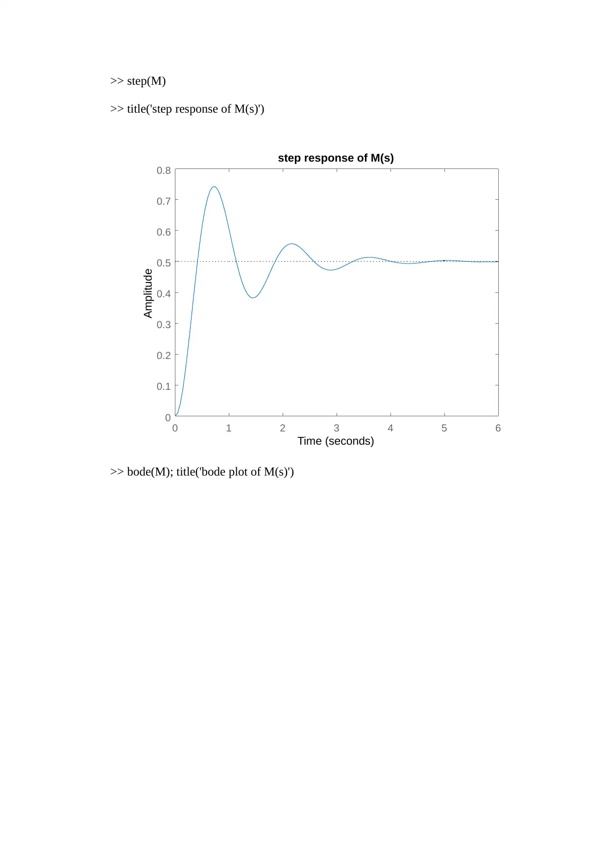
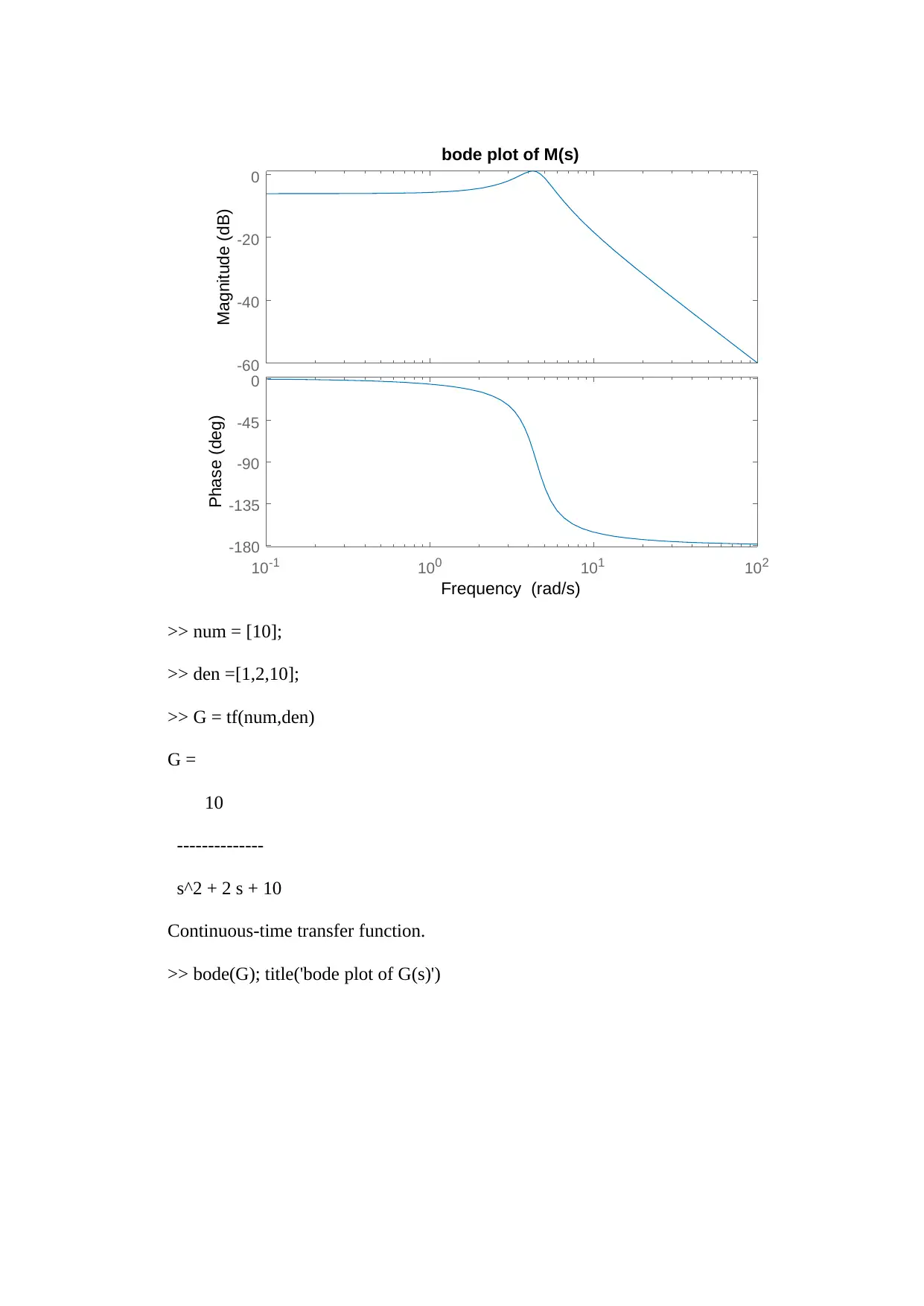
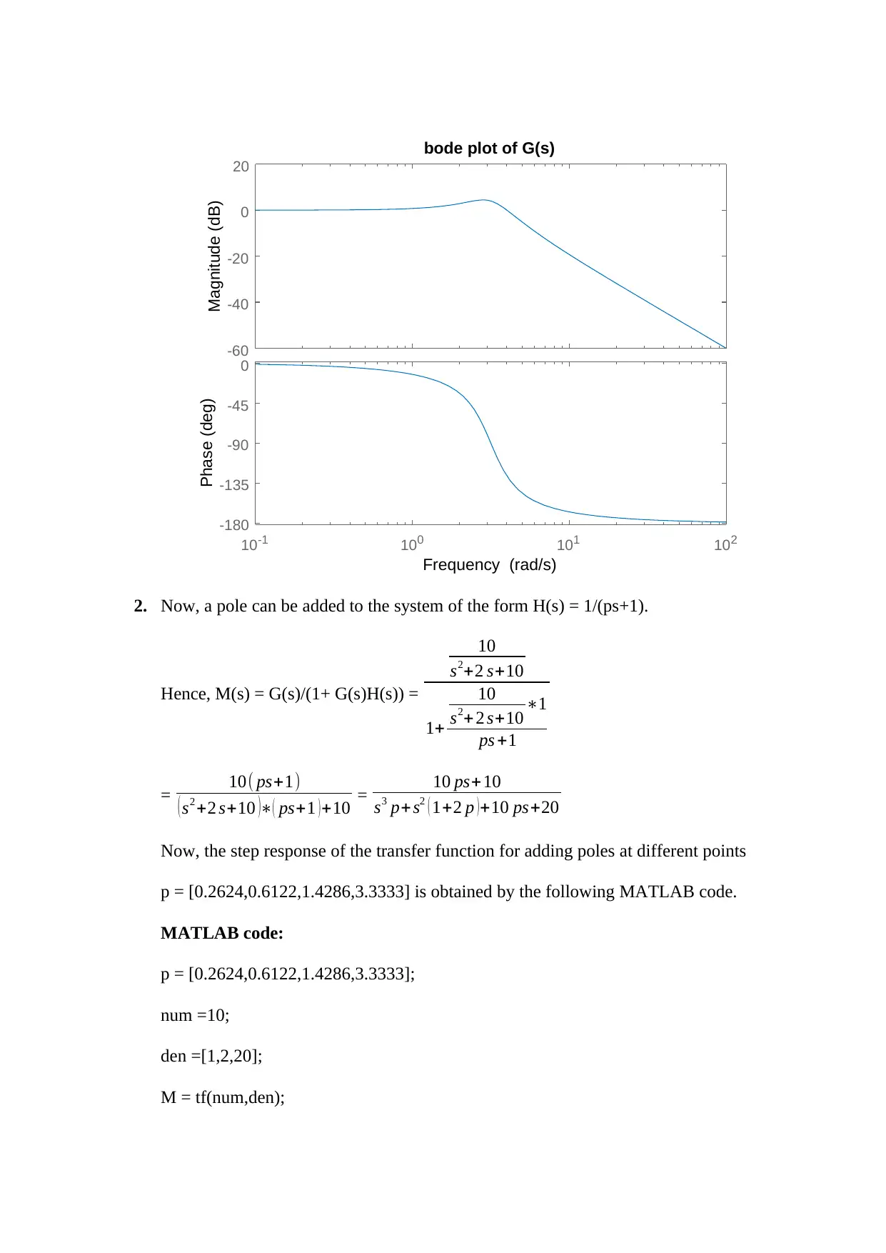
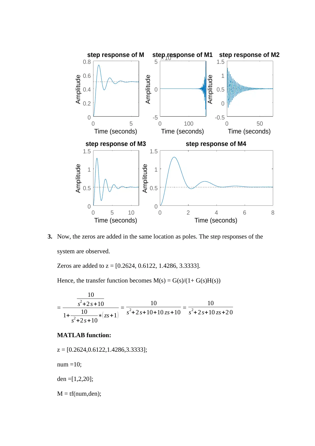
This project analyzes the effects of adding poles and zeros to a second-order transfer function within a control system. The project utilizes MATLAB to simulate and analyze the impact of these additions on the system's step response, Bode plots, and key performance indicators. The analysis covers the effects of adding poles and zeros separately, examining how they influence parameters such as peak overshoot, rise time, phase margin, bandwidth, and gain crossover frequency. The project includes MATLAB code snippets, plots of step responses, Bode plots and tabular data to illustrate the observed effects and relationships between these parameters, providing a comprehensive understanding of the impact of pole and zero placement on system stability and performance. The project concludes by summarizing the observed relationships between the system properties and the addition of poles and zeros.

1. The control system is given by the following block diagram.
Here, G ( s ) = 10
s2 +2 s+10
G(s) is the open loop transfer function and M(s) is the closed loop transfer function
given by,
M(s) = G(s)H(s)/ (1 + G(s)H(s))
Now, with no addition of poles and zero H(s) = 1 is considered here.
So, M(s) = G(s)/(1+G(s)) ¿ 10
s2+2 s+20
Now, the step response and Bode plot of M(s) are shown below.
>> num =[10];
>> den =[1,2,20];
>> M = tf(num,den)
M =
10
--------------
s^2 + 2 s + 20
Continuous-time transfer function.

>> step(M)
>> title('step response of M(s)')
0 1 2 3 4 5 6
0
0.1
0.2
0.3
0.4
0.5
0.6
0.7
0.8
step response of M(s)
Time (seconds)
Amplitude
>> bode(M); title('bode plot of M(s)')

-60
-40
-20
0
Magnitude (dB)
10-1 100 101 102
-180
-135
-90
-45
0
Phase (deg)
bode plot of M(s)
Frequency (rad/s)
>> num = [10];
>> den =[1,2,10];
>> G = tf(num,den)
G =
10
--------------
s^2 + 2 s + 10
Continuous-time transfer function.
>> bode(G); title('bode plot of G(s)')

-60
-40
-20
0
20
Magnitude (dB)
10-1 100 101 102
-180
-135
-90
-45
0
Phase (deg)
bode plot of G(s)
Frequency (rad/s)
2. Now, a pole can be added to the system of the form H(s) = 1/(ps+1).
Hence, M(s) = G(s)/(1+ G(s)H(s)) =
10
s2+2 s+10
1+
10
s2+ 2 s+10 ∗1
ps +1
= 10( ps+1)
( s2 +2 s+10 )∗( ps+1 )+10 = 10 ps+ 10
s3 p+ s2 ( 1+2 p )+10 ps+20
Now, the step response of the transfer function for adding poles at different points
p = [0.2624,0.6122,1.4286,3.3333] is obtained by the following MATLAB code.
MATLAB code:
p = [0.2624,0.6122,1.4286,3.3333];
num =10;
den =[1,2,20];
M = tf(num,den);

num1 = [10*p(1),10];
den1 = [p(1),(1+2*p(1)),10*p(1),20];
M1 = tf(num1,den1);
num2 = [10*p(2),10];
den2 = [p(2),(1+2*p(2)),10*p(2),20];
M2 = tf(num2,den2);
num3 = [10*p(3),10];
den3 = [p(3),(1+2*p(3)),10*p(3),20];
M3 = tf(num3,den3);
num4 = [10*p(4),10];
den4 = [p(4),(1+2*p(4)),10*p(4),20];
M4 = tf(num4,den4);
subplot(2,3,1)
step(M); title('step response of M')
subplot(2,3,2)
step(M1); title('step response of M1')
subplot(2,3,3)
step(M2); title('step response of M2')
subplot(2,3,4)
step(M3); title('step response of M3')
subplot(2,3,[5,6])
step(M4); title('step response of M4')
Plot:

0 5
0
0.2
0.4
0.6
0.8
step response of M
Time (seconds)
Amplitude
0 100
-5
0
5 10 12step response of M1
Time (seconds)
Amplitude
0 50
-0.5
0
0.5
1
1.5
step response of M2
Time (seconds)
Amplitude
0 5 10
0
0.5
1
1.5
step response of M3
Time (seconds)
Amplitude
0 2 4 6 8
0
0.5
1
1.5
step response of M4
Time (seconds)
Amplitude
3. Now, the zeros are added in the same location as poles. The step responses of the
system are observed.
Zeros are added to z = [0.2624, 0.6122, 1.4286, 3.3333].
Hence, the transfer function becomes M(s) = G(s)/(1+ G(s)H(s))
=
10
s2 +2 s +10
1+ 10
s2 +2 s +10∗( zs +1 )
= 10
s2+2 s+10+10 zs +10 = 10
s2+ 2 s+10 zs +2 0
MATLAB function:
z = [0.2624,0.6122,1.4286,3.3333];
num =10;
den =[1,2,20];
M = tf(num,den);

num1 = 10;
den1 = [1,(10*z(1)+2),20];
M1 = tf(num1,den1);
num2 = 10;
den2 = [1,(10*z(2)+2),20];
M2 = tf(num2,den2);
num3 = 10;
den3 = [1,(10*z(3)+2),20];
M3 = tf(num3,den3);
num4 = 10;
den4 = [1,(10*z(4)+2),20];
M4 = tf(num4,den4);
subplot(2,3,1)
step(M); title('step response of M')
subplot(2,3,2)
step(M1); title('step response of M1')
subplot(2,3,3)
step(M2); title('step response of M2')
subplot(2,3,4)
step(M3); title('step response of M3')
subplot(2,3,[5,6])
step(M4); title('step response of M4')
Plot:

0 5
0
0.2
0.4
0.6
0.8
step response of M
Time (seconds)
Amplitude
0 1 2 3
0
0.2
0.4
0.6
step response of M1
Time (seconds)
Amplitude
0 1
0
0.2
0.4
0.6
step response of M2
Time (seconds)
Amplitude
0 2 4
0
0.2
0.4
0.6
step response of M3
Time (seconds)
Amplitude
0 2 4 6 8 10 12
0
0.2
0.4
0.6
step response of M4
Time (seconds)
Amplitude
4. Now, addition of poles how affects the Peak Overshoot (POS), risetime (Tr), Phase
margin (PM) and Bandwidth (BW) of the system is observed and recorded in a table.
Now, the bandwidth of the system can be obtained by using the bandwidth function in
MATLAB.
MATLAB code for bandwidth:
p = [0.2624,0.6122,1.4286,3.3333];
num =10;
den =[1,2,20];
M = tf(num,den);
num1 = [10*p(1),10];
den1 = [p(1),(1+2*p(1)),10*p(1),20];
M1 = tf(num1,den1);
num2 = [10*p(2),10];

den2 = [p(2),(1+2*p(2)),10*p(2),20];
M2 = tf(num2,den2);
num3 = [10*p(3),10];
den3 = [p(3),(1+2*p(3)),10*p(3),20];
M3 = tf(num3,den3);
num4 = [10*p(4),10];
den4 = [p(4),(1+2*p(4)),10*p(4),20];
M4 = tf(num4,den4);
b = bandwidth(M);
b1 = bandwidth(M1);
b2 = bandwidth(M2);
b3 = bandwidth(M3);
b4 = bandwidth(M4);
b
b1
b2
b3
b4
Output:
b =
6.6987
b1 =
5.9561
b2 =
5.8879

b3 =
5.9148
b4 =
5.9412
Risetime (Tr) : Rise time is the time required for the response to reach from 10% to
90% of the steady-state value.
Peak Overshoot: The maximum value attained by the response.
Phase margin: The difference between the phase angle of the transfer function and
180° obtained at gain crossover frequency. The gain and phase margin can be directly
obtained from MATLAB.
[Gm,Pm] = margin(M)
Gm =
Inf
Pm =
73.1630
>> [Gm,Pm]=margin(M1)
Gm =
0.9064
Pm =
1.1538
>> [Gm,Pm]=margin(M2)
Gm =
Inf
Pm =
23.1292

>> [Gm,Pm]=margin(M3)
Gm =
Inf
Pm =
38.8916
>> [Gm,Pm]=margin(M4)
Gm =
Inf
Pm =
46.8169
Furthermore, the stepinfo function in MATLAB all the properties of the step response
of the system.
stepinfo(M)
ans =
struct with fields:
RiseTime: 0.2767
SettlingTime: 3.7804
SettlingMin: 0.3819
SettlingMax: 0.7426
Overshoot: 48.5150
Undershoot: 0

Peak: 0.7426
PeakTime: 0.7368
>> stepinfo(M2)
ans =
struct with fields:
RiseTime: 0.2448
SettlingTime: 47.0894
SettlingMin: -0.1796
SettlingMax: 1.2519
Overshoot: 150.3718
Undershoot: 35.9181
Peak: 1.2519
PeakTime: 0.9032
Items – effect of adding
pole
Results/Comments
POS From the graphs it is
observed that POS is
increased when a pole is
added to G(s).
Tr The risetime decreases.
PM Phase margin also