ECOM058 Applied Econometrics Assignment: UK Money Demand Analysis
VerifiedAdded on 2023/02/01
|34
|7312
|97
Homework Assignment
AI Summary
This assignment analyzes the money demand function in the UK, examining both short-run and long-run dynamics. The solution begins with estimating a static money demand function using inflation rate, real GDP, and interest rate as independent variables. Autocorrelation tests are performed to assess model robustness. The analysis then shifts to the long run, acknowledging the challenges of directly observing the money demand function and employing instrumental variables to address potential endogeneity issues. The solution includes unit root tests using the Augmented Dickey-Fuller test and cointegration analysis using the Engel-Granger test. The document provides detailed regression results, interpretations of coefficients, and statistical tests, including F-tests and LM tests for autocorrelation. The assignment also discusses the impact of autocorrelation on OLS estimators and the implications for policy formulation.

Running head: APPLIED ECONOMETRICS
Applied Econometrics
Name of the Student
Name of the University
Course ID
Applied Econometrics
Name of the Student
Name of the University
Course ID
Paraphrase This Document
Need a fresh take? Get an instant paraphrase of this document with our AI Paraphraser
1APPLIED ECONOMETRICS
Executive Summary
The paper aims to analyze the money demand function both in the short run and in the long run.
The static money demand function has been estimated taking inflation rate, real GDP and interest
rate. In order to analyze robustness of the model autocorrelation test has been performed for
examining presence of serial correlation in the model. Condition in the short run however is
different from that in the long run. In the long run, it is assumed that money demand function is
not directly observable and difference between observed money supply tends to adjust towards
the expected difference in money supply having certain speed of adjustment. In the long run
inclusion of lagged dependent variables may result in the problem of endogeneity where
independent variables are found to be related with the error term. In order to eliminate the
problem of endogeneity the technique of instrumental variables is used through the estimation
method of two stage least square. Each of the series has been tested for unit root by employing
the Augmenyed Dicky Fuller test. Finally, Engel Granger test has been performed to examine co-
integration among the variables. The money demand function and its associate determinants
provide useful implication for policy formulation.
2APPLIED ECONOMETRICS
Table of Contents
Question 1........................................................................................................................................4
Question 2........................................................................................................................................6
Question a....................................................................................................................................6
Question b....................................................................................................................................7
Question c....................................................................................................................................8
Question 3........................................................................................................................................8
Question a....................................................................................................................................8
Question b....................................................................................................................................9
Question 4......................................................................................................................................10
Question a..................................................................................................................................10
Question b..................................................................................................................................12
Question c..................................................................................................................................12
Question 5......................................................................................................................................13
Question a..................................................................................................................................13
Question b..................................................................................................................................13
Question c..................................................................................................................................13
Question d..................................................................................................................................13
Question 6......................................................................................................................................14
Question 7......................................................................................................................................15
⊘ This is a preview!⊘
Do you want full access?
Subscribe today to unlock all pages.
Trusted by 1+ million students worldwide
3APPLIED ECONOMETRICS
Question a..................................................................................................................................15
Question b..................................................................................................................................15
Question c..................................................................................................................................15
Question 8......................................................................................................................................15
Question a..................................................................................................................................15
Question b..................................................................................................................................16
Question c..................................................................................................................................16
Question 9......................................................................................................................................16
Question a..................................................................................................................................16
Question b..................................................................................................................................18
Question c..................................................................................................................................18
Question 10....................................................................................................................................18
References and Bibliography.........................................................................................................20
Appendix........................................................................................................................................22
Question a..................................................................................................................................15
Question b..................................................................................................................................15
Question c..................................................................................................................................15
Question 8......................................................................................................................................15
Question a..................................................................................................................................15
Question b..................................................................................................................................16
Question c..................................................................................................................................16
Question 9......................................................................................................................................16
Question a..................................................................................................................................16
Question b..................................................................................................................................18
Question c..................................................................................................................................18
Question 10....................................................................................................................................18
References and Bibliography.........................................................................................................20
Appendix........................................................................................................................................22
Paraphrase This Document
Need a fresh take? Get an instant paraphrase of this document with our AI Paraphraser
4APPLIED ECONOMETRICS
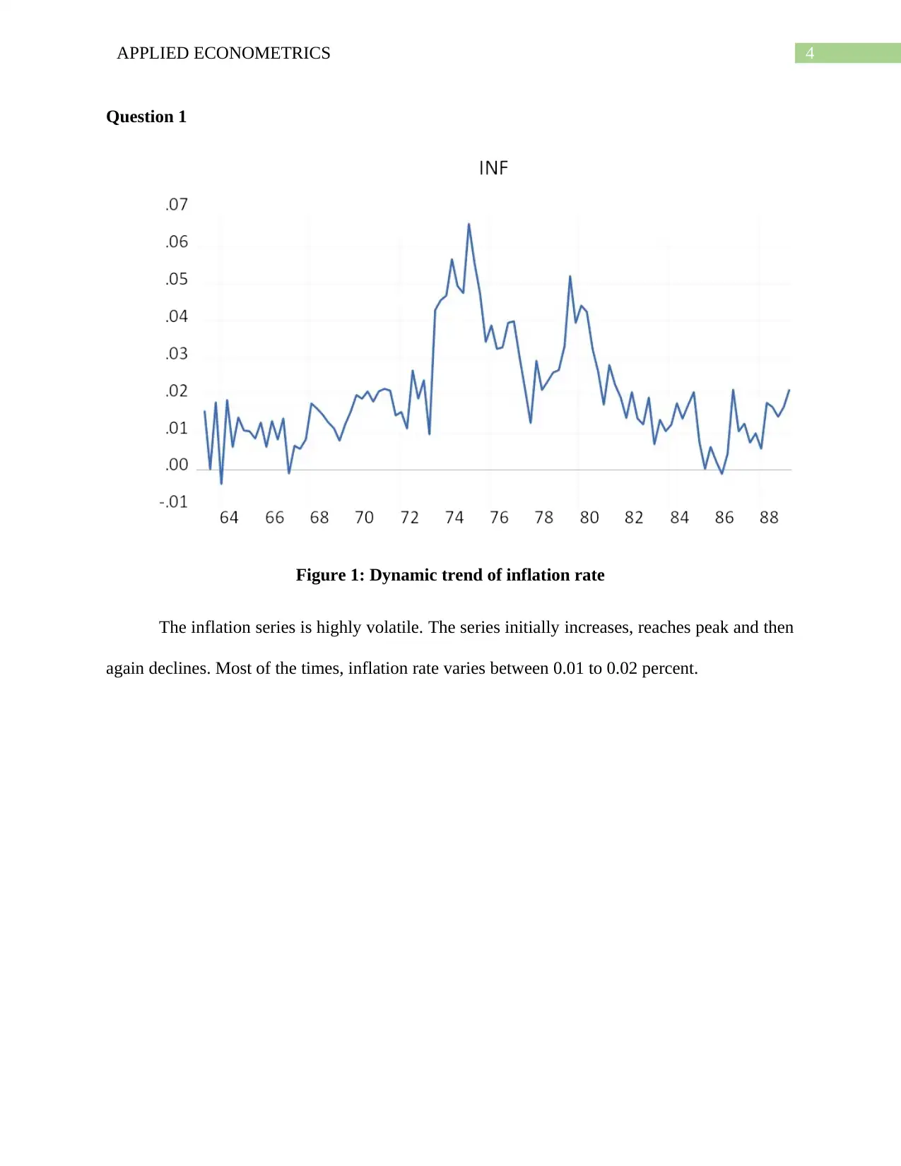
Question 1
Figure 1: Dynamic trend of inflation rate
The inflation series is highly volatile. The series initially increases, reaches peak and then
again declines. Most of the times, inflation rate varies between 0.01 to 0.02 percent.
Question 1
Figure 1: Dynamic trend of inflation rate
The inflation series is highly volatile. The series initially increases, reaches peak and then
again declines. Most of the times, inflation rate varies between 0.01 to 0.02 percent.
5APPLIED ECONOMETRICS
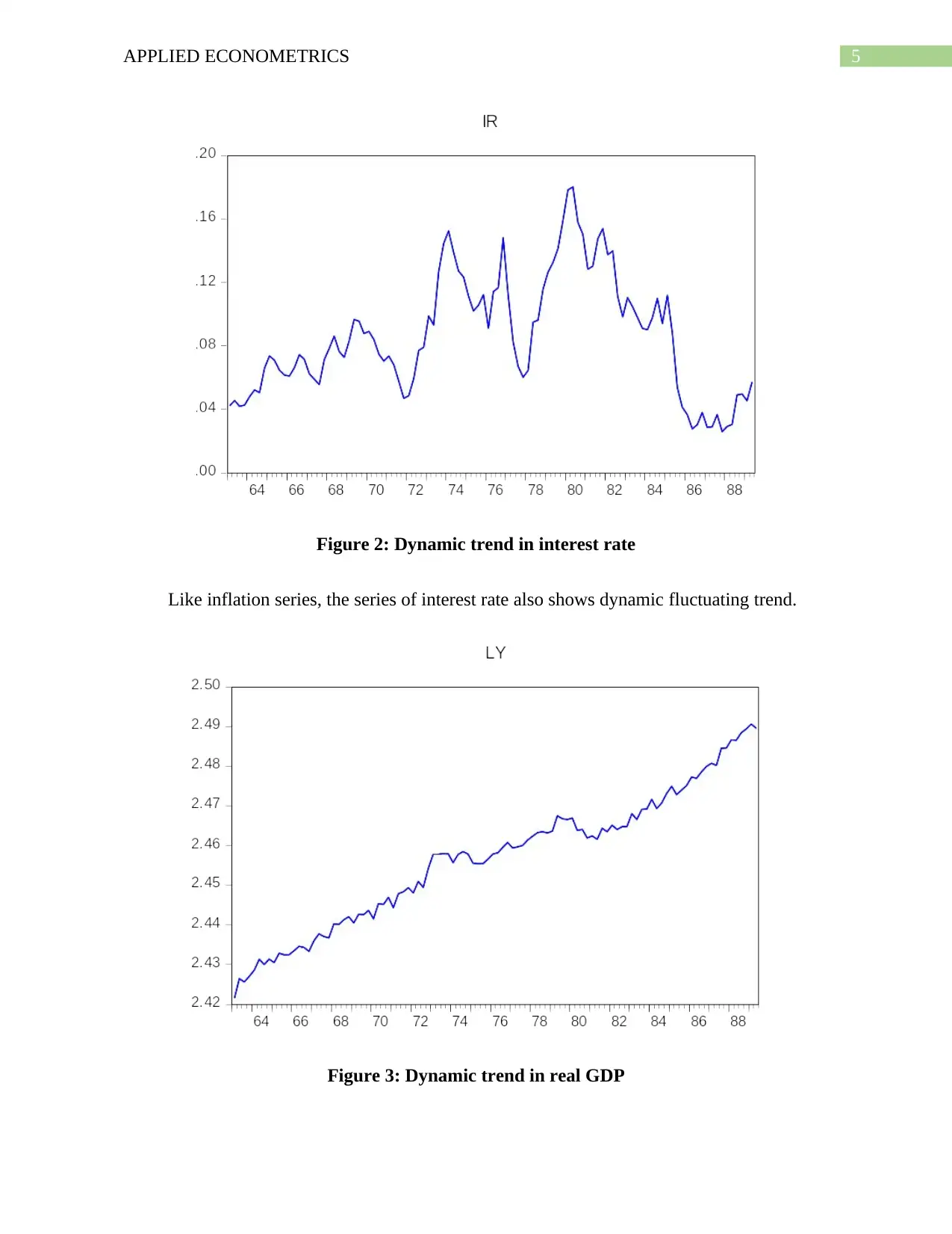
Figure 2: Dynamic trend in interest rate
Like inflation series, the series of interest rate also shows dynamic fluctuating trend.
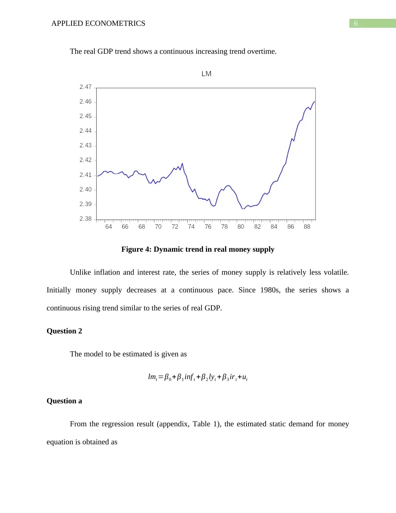
Figure 3: Dynamic trend in real GDP
Figure 2: Dynamic trend in interest rate
Like inflation series, the series of interest rate also shows dynamic fluctuating trend.
Figure 3: Dynamic trend in real GDP
⊘ This is a preview!⊘
Do you want full access?
Subscribe today to unlock all pages.
Trusted by 1+ million students worldwide
6APPLIED ECONOMETRICS
The real GDP trend shows a continuous increasing trend overtime.
Figure 4: Dynamic trend in real money supply
Unlike inflation and interest rate, the series of money supply is relatively less volatile.
Initially money supply decreases at a continuous pace. Since 1980s, the series shows a
continuous rising trend similar to the series of real GDP.
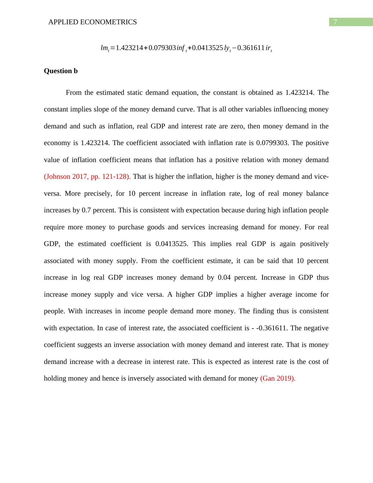
Question 2
The model to be estimated is given as
lmt =β0 +β1 inf t +β2 lyt +β3 irt +ut
Question a
From the regression result (appendix, Table 1), the estimated static demand for money
equation is obtained as
The real GDP trend shows a continuous increasing trend overtime.
Figure 4: Dynamic trend in real money supply
Unlike inflation and interest rate, the series of money supply is relatively less volatile.
Initially money supply decreases at a continuous pace. Since 1980s, the series shows a
continuous rising trend similar to the series of real GDP.
Question 2
The model to be estimated is given as
lmt =β0 +β1 inf t +β2 lyt +β3 irt +ut
Question a
From the regression result (appendix, Table 1), the estimated static demand for money
equation is obtained as
Paraphrase This Document
Need a fresh take? Get an instant paraphrase of this document with our AI Paraphraser
7APPLIED ECONOMETRICS
lmt =1.423214+0.079303inf t +0.0413525 lyt −0.361611 irt
Question b
From the estimated static demand equation, the constant is obtained as 1.423214. The
constant implies slope of the money demand curve. That is all other variables influencing money
demand and such as inflation, real GDP and interest rate are zero, then money demand in the
economy is 1.423214. The coefficient associated with inflation rate is 0.0799303. The positive
value of inflation coefficient means that inflation has a positive relation with money demand
(Johnson 2017, pp. 121-128). That is higher the inflation, higher is the money demand and vice-
versa. More precisely, for 10 percent increase in inflation rate, log of real money balance
increases by 0.7 percent. This is consistent with expectation because during high inflation people
require more money to purchase goods and services increasing demand for money. For real
GDP, the estimated coefficient is 0.0413525. This implies real GDP is again positively
associated with money supply. From the coefficient estimate, it can be said that 10 percent
increase in log real GDP increases money demand by 0.04 percent. Increase in GDP thus
increase money supply and vice versa. A higher GDP implies a higher average income for
people. With increases in income people demand more money. The finding thus is consistent
with expectation. In case of interest rate, the associated coefficient is - -0.361611. The negative
coefficient suggests an inverse association with money demand and interest rate. That is money
demand increase with a decrease in interest rate. This is expected as interest rate is the cost of
holding money and hence is inversely associated with demand for money (Gan 2019).
8APPLIED ECONOMETRICS
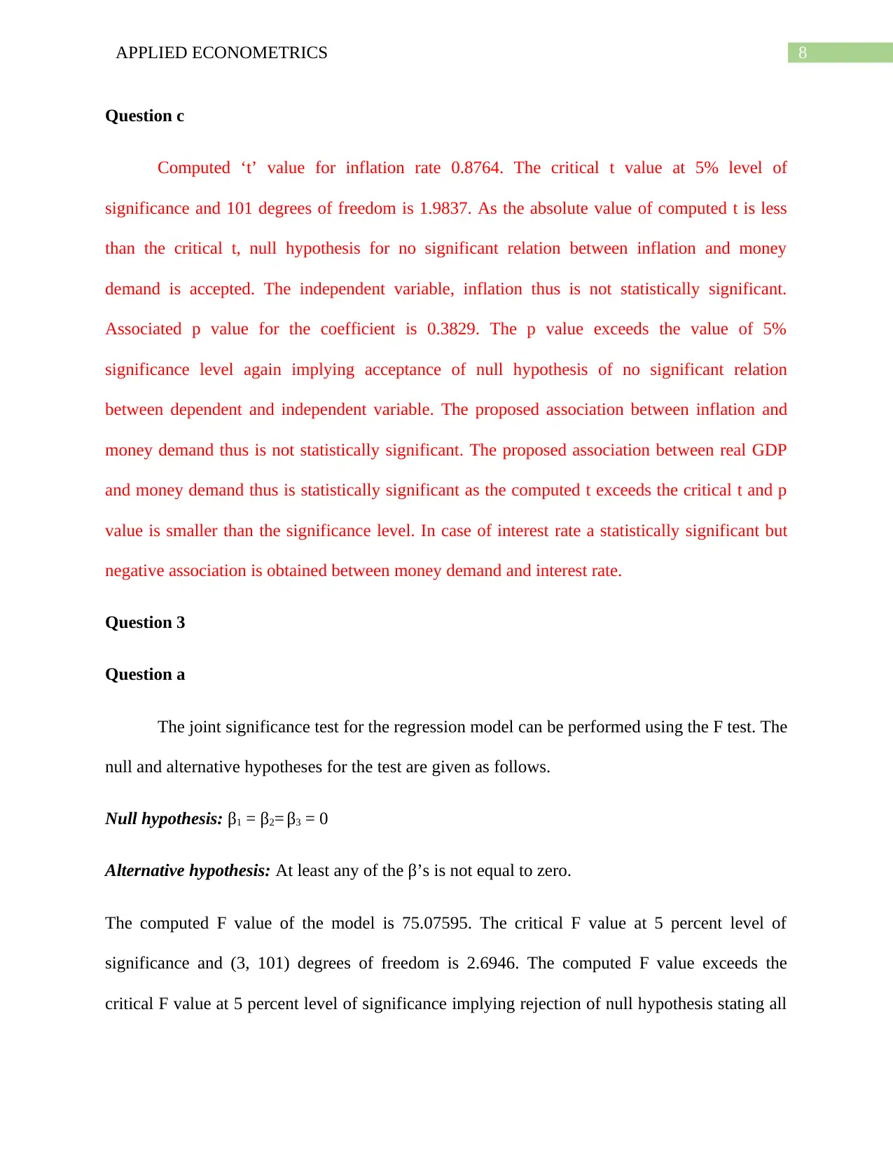
Question c
Computed ‘t’ value for inflation rate 0.8764. The critical t value at 5% level of
significance and 101 degrees of freedom is 1.9837. As the absolute value of computed t is less
than the critical t, null hypothesis for no significant relation between inflation and money
demand is accepted. The independent variable, inflation thus is not statistically significant.
Associated p value for the coefficient is 0.3829. The p value exceeds the value of 5%
significance level again implying acceptance of null hypothesis of no significant relation
between dependent and independent variable. The proposed association between inflation and
money demand thus is not statistically significant. The proposed association between real GDP
and money demand thus is statistically significant as the computed t exceeds the critical t and p
value is smaller than the significance level. In case of interest rate a statistically significant but
negative association is obtained between money demand and interest rate.
Question 3
Question a
The joint significance test for the regression model can be performed using the F test. The
null and alternative hypotheses for the test are given as follows.
Null hypothesis: β1 = β2= β3 = 0
Alternative hypothesis: At least any of the β’s is not equal to zero.
The computed F value of the model is 75.07595. The critical F value at 5 percent level of
significance and (3, 101) degrees of freedom is 2.6946. The computed F value exceeds the
critical F value at 5 percent level of significance implying rejection of null hypothesis stating all
⊘ This is a preview!⊘
Do you want full access?
Subscribe today to unlock all pages.
Trusted by 1+ million students worldwide
9APPLIED ECONOMETRICS
coefficients are zero. This can therefore be said that at least one of the coefficient is significantly
different from zero and hence, the model is jointly significant. The result is again supported by
the p value test. Associated p value for the F statistics is 0.0000. As the p value is less than
significance value of 0.05, the null hypothesis stating that the overall model is insignificant is
rejected. The independent variables in the model thus are jointly significant.
Question b
In multiple regression model adjusted R square is used as a measure of goodness of fit.
The obtained value of adjusted R square is 0.6812. The value indicates that inflation, real GDP
and interest rate can together explain 68 percent variation of the dependent variables. As the
independent variables account a considerably higher variability of the dependent variable, the
model is a good fit model.
Paraphrase This Document
Need a fresh take? Get an instant paraphrase of this document with our AI Paraphraser
10APPLIED ECONOMETRICS
Question 4
Question a
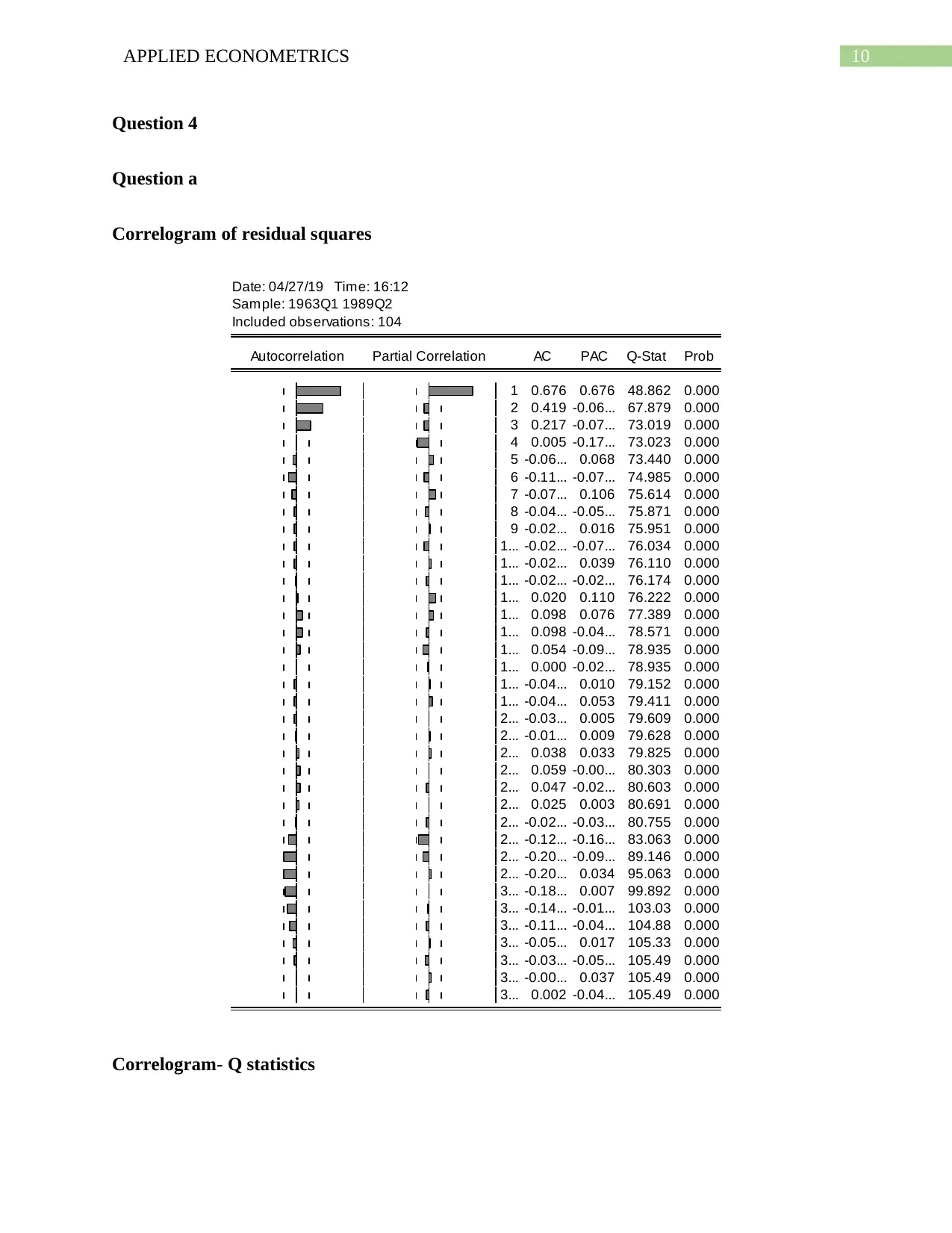
Correlogram of residual squares
Date: 04/27/19 Time: 16:12
Sample: 1963Q1 1989Q2
Included observations: 104
Autocorrelation Partial Correlation AC PAC Q-Stat Prob
1 0.676 0.676 48.862 0.000
2 0.419 -0.06... 67.879 0.000
3 0.217 -0.07... 73.019 0.000
4 0.005 -0.17... 73.023 0.000
5 -0.06... 0.068 73.440 0.000
6 -0.11... -0.07... 74.985 0.000
7 -0.07... 0.106 75.614 0.000
8 -0.04... -0.05... 75.871 0.000
9 -0.02... 0.016 75.951 0.000
1... -0.02... -0.07... 76.034 0.000
1... -0.02... 0.039 76.110 0.000
1... -0.02... -0.02... 76.174 0.000
1... 0.020 0.110 76.222 0.000
1... 0.098 0.076 77.389 0.000
1... 0.098 -0.04... 78.571 0.000
1... 0.054 -0.09... 78.935 0.000
1... 0.000 -0.02... 78.935 0.000
1... -0.04... 0.010 79.152 0.000
1... -0.04... 0.053 79.411 0.000
2... -0.03... 0.005 79.609 0.000
2... -0.01... 0.009 79.628 0.000
2... 0.038 0.033 79.825 0.000
2... 0.059 -0.00... 80.303 0.000
2... 0.047 -0.02... 80.603 0.000
2... 0.025 0.003 80.691 0.000
2... -0.02... -0.03... 80.755 0.000
2... -0.12... -0.16... 83.063 0.000
2... -0.20... -0.09... 89.146 0.000
2... -0.20... 0.034 95.063 0.000
3... -0.18... 0.007 99.892 0.000
3... -0.14... -0.01... 103.03 0.000
3... -0.11... -0.04... 104.88 0.000
3... -0.05... 0.017 105.33 0.000
3... -0.03... -0.05... 105.49 0.000
3... -0.00... 0.037 105.49 0.000
3... 0.002 -0.04... 105.49 0.000
Correlogram- Q statistics
Question 4
Question a
Correlogram of residual squares
Date: 04/27/19 Time: 16:12
Sample: 1963Q1 1989Q2
Included observations: 104
Autocorrelation Partial Correlation AC PAC Q-Stat Prob
1 0.676 0.676 48.862 0.000
2 0.419 -0.06... 67.879 0.000
3 0.217 -0.07... 73.019 0.000
4 0.005 -0.17... 73.023 0.000
5 -0.06... 0.068 73.440 0.000
6 -0.11... -0.07... 74.985 0.000
7 -0.07... 0.106 75.614 0.000
8 -0.04... -0.05... 75.871 0.000
9 -0.02... 0.016 75.951 0.000
1... -0.02... -0.07... 76.034 0.000
1... -0.02... 0.039 76.110 0.000
1... -0.02... -0.02... 76.174 0.000
1... 0.020 0.110 76.222 0.000
1... 0.098 0.076 77.389 0.000
1... 0.098 -0.04... 78.571 0.000
1... 0.054 -0.09... 78.935 0.000
1... 0.000 -0.02... 78.935 0.000
1... -0.04... 0.010 79.152 0.000
1... -0.04... 0.053 79.411 0.000
2... -0.03... 0.005 79.609 0.000
2... -0.01... 0.009 79.628 0.000
2... 0.038 0.033 79.825 0.000
2... 0.059 -0.00... 80.303 0.000
2... 0.047 -0.02... 80.603 0.000
2... 0.025 0.003 80.691 0.000
2... -0.02... -0.03... 80.755 0.000
2... -0.12... -0.16... 83.063 0.000
2... -0.20... -0.09... 89.146 0.000
2... -0.20... 0.034 95.063 0.000
3... -0.18... 0.007 99.892 0.000
3... -0.14... -0.01... 103.03 0.000
3... -0.11... -0.04... 104.88 0.000
3... -0.05... 0.017 105.33 0.000
3... -0.03... -0.05... 105.49 0.000
3... -0.00... 0.037 105.49 0.000
3... 0.002 -0.04... 105.49 0.000
Correlogram- Q statistics
11APPLIED ECONOMETRICS
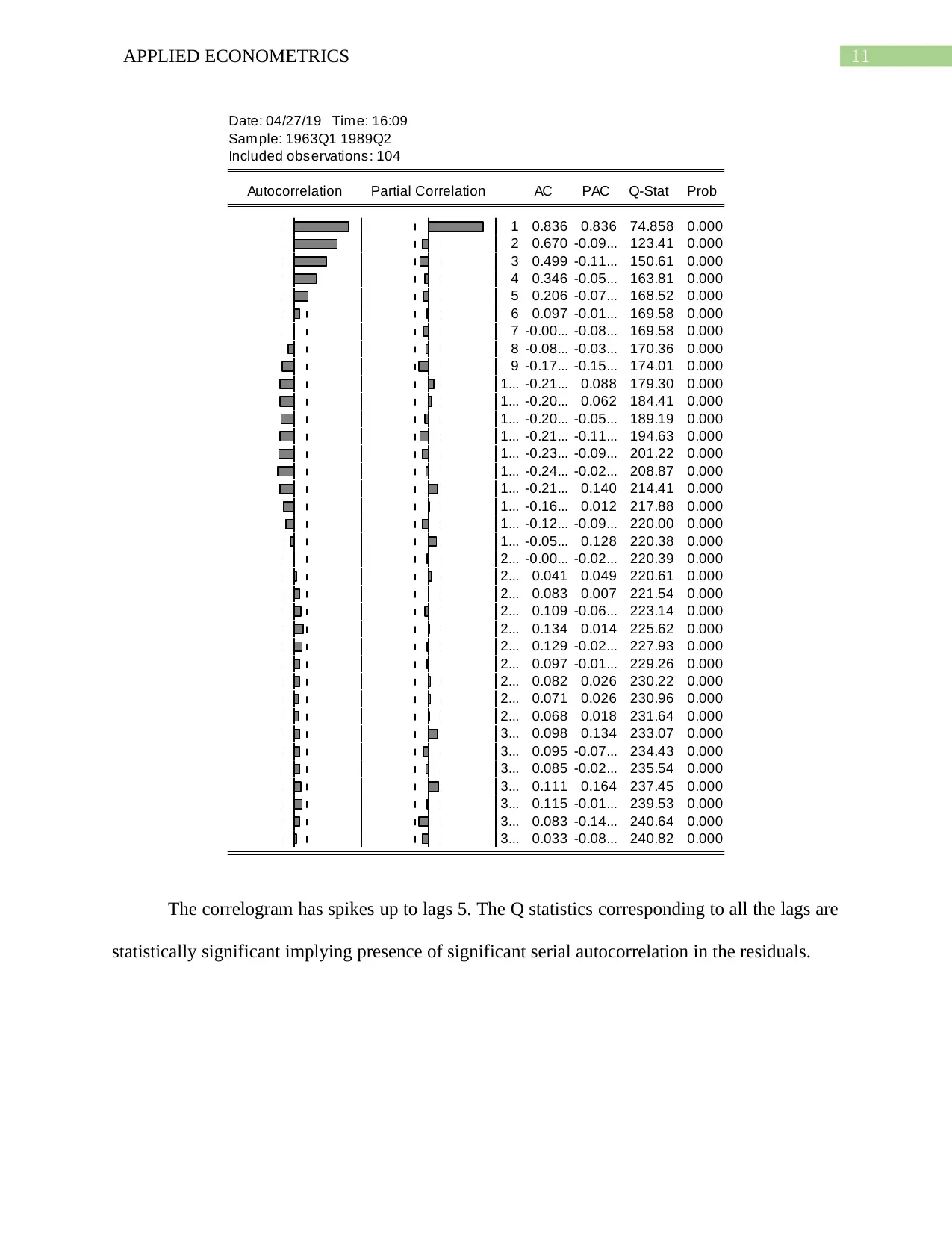
Date: 04/27/19 Time: 16:09
Sample: 1963Q1 1989Q2
Included observations: 104
Autocorrelation Partial Correlation AC PAC Q-Stat Prob
1 0.836 0.836 74.858 0.000
2 0.670 -0.09... 123.41 0.000
3 0.499 -0.11... 150.61 0.000
4 0.346 -0.05... 163.81 0.000
5 0.206 -0.07... 168.52 0.000
6 0.097 -0.01... 169.58 0.000
7 -0.00... -0.08... 169.58 0.000
8 -0.08... -0.03... 170.36 0.000
9 -0.17... -0.15... 174.01 0.000
1... -0.21... 0.088 179.30 0.000
1... -0.20... 0.062 184.41 0.000
1... -0.20... -0.05... 189.19 0.000
1... -0.21... -0.11... 194.63 0.000
1... -0.23... -0.09... 201.22 0.000
1... -0.24... -0.02... 208.87 0.000
1... -0.21... 0.140 214.41 0.000
1... -0.16... 0.012 217.88 0.000
1... -0.12... -0.09... 220.00 0.000
1... -0.05... 0.128 220.38 0.000
2... -0.00... -0.02... 220.39 0.000
2... 0.041 0.049 220.61 0.000
2... 0.083 0.007 221.54 0.000
2... 0.109 -0.06... 223.14 0.000
2... 0.134 0.014 225.62 0.000
2... 0.129 -0.02... 227.93 0.000
2... 0.097 -0.01... 229.26 0.000
2... 0.082 0.026 230.22 0.000
2... 0.071 0.026 230.96 0.000
2... 0.068 0.018 231.64 0.000
3... 0.098 0.134 233.07 0.000
3... 0.095 -0.07... 234.43 0.000
3... 0.085 -0.02... 235.54 0.000
3... 0.111 0.164 237.45 0.000
3... 0.115 -0.01... 239.53 0.000
3... 0.083 -0.14... 240.64 0.000
3... 0.033 -0.08... 240.82 0.000
The correlogram has spikes up to lags 5. The Q statistics corresponding to all the lags are
statistically significant implying presence of significant serial autocorrelation in the residuals.
⊘ This is a preview!⊘
Do you want full access?
Subscribe today to unlock all pages.
Trusted by 1+ million students worldwide
1 out of 34
Related Documents


Your All-in-One AI-Powered Toolkit for Academic Success.
+13062052269
info@desklib.com
Available 24*7 on WhatsApp / Email
![[object Object]](/_next/static/media/star-bottom.7253800d.svg)
Unlock your academic potential
Copyright © 2020–2026 A2Z Services. All Rights Reserved. Developed and managed by ZUCOL.