Monte Carlo Integration and Variance Analysis: A Statistical Project

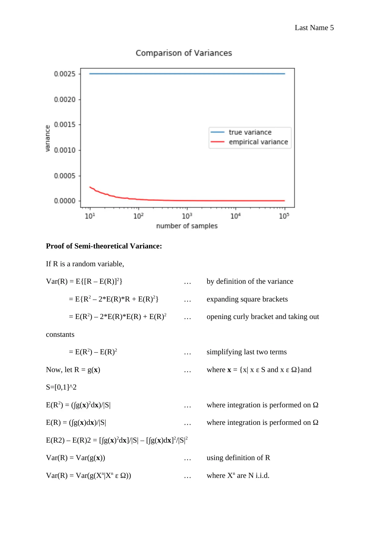
This project uses Monte Carlo methods to perform statistical analysis and integral estimation. The assignment begins with generating random coordinates and plotting them in 2D and 3D spaces. It then calculates the integral of a function over a specified region using Monte Carlo techniques. The project includes estimating the value of Pi using this method and analyzing the mean and standard deviation of the estimated integrals for different sample sizes. The analysis involves plotting the mean and standard deviation as a function of sample size, and determining the sample size required for the standard deviation to be within a certain percentage of the mean. The project also compares theoretical and empirical variances and provides a proof of a semi-theoretical variance formula. Python code is provided for all tasks, including plotting and numerical computations, alongside detailed explanations of the methodology and results. The project showcases the application of Monte Carlo methods in statistical analysis and numerical integration.

Last Name 1
Name:
Professor:
Course:
Date:
Project 1
Q1) Generation of N two-dimensional random co-ordinates in [0, 1]^2:
There is a direct instruction available in “numpy” for this task:
X = np.random.rand(N, 2)
To ensure reproducibility of the results, following command requires to be provided,
np.random.seed(1234) where 1234 is any arbitrary number.
Q2) 3D-Plot of g values over [0, 1]^2:
Purple points are valid points in the region Ω = (H>=0). Yellow points are not in Ω.

Last Name 2
Q3) Code for calculating integral of g over region Ω:
def my_Monte_Carlo():
X = np.random.rand(n, 2)
H = my_h_function(X)
G = my_g_function(X)
C = H >= 0
return sum(G*C)/n
The value of the integral is 0.03441.
Q4) Value of Pi by Monte Carlo Method:
def my_g_function(X):
m = len(X)
return np.array([1 for i1 in range(m)])
def my_h_function(X):
output = []
for x in X:
x1, x2 = x
output.append(1 - x1**2 - x2**2)
return np.array(output)
n = 1000
np.random.seed(1234)
print("Estimate of Pi with 1000 pairs of random numbers", 4*my_Monte_Carlo())
Value of Pi is obtained as 3.128 (actual 3.142)
Q5) a) Mean and Standard Deviation for N=1000 and T=500
Mean = 0.03151
Standard Deviation = 0.001719
b) Plot of Mean and Standard Deviations for Nset Samples
# Q5(B) Mean and Standard deviation plots
Nset = np.round(np.logspace(1, 5, 100))
I, t0 = [], time.clock()
np.random.seed(1234)
for i in range(100):

Last Name 3
print(i, time.clock()-t0)
n = int(Nset[i])
J = []
for t in range(500):
J.append(my_Monte_Carlo())
I.append(np.array(J))
I = np.array(I)
plt.figure ()
plt.semilogx (Nset, I, 'kx')
plt.semilogx (Nset, np.mean(I, 1), 'b', label = 'mean')
plt.semilogx (Nset, np.mean(I, 1) + np.std(I, 1), 'r', label = 'mean +/- stdev')
plt.semilogx (Nset, np.mean(I, 1) - np.std (I, 1) , 'r')
plt.xlabel('number of samples')
plt.ylabel('estimated integral')
plt.legend()
plt.savefig("Q5.png")
Plot of Mean and Standard Deviation as Function of Sample Size

Last Name 4
For number of samples >= 1150, the standard deviation is within 5% of mean value.
This value can be calculated using the following commands:
m = list(np.mean(I, 1)*0.05 >= np.std(I, 1)).index(True)
print(Nset[m])
Q6) Code and Plot
def my_g_function(X):
output = []
for x in X:
x1, x2 = x
output.append(0.5/math.pi*math.exp(-0.5*(x1**2 + x2**2)))
output = np.array(output)
output = output*output
return output
n = int(1e5)
np.random.seed(1234)
v2 = my_Monte_Carlo()
v = v2 - Intg*Intg
print("Variance for N = 100,000:", v)
V = np.array([v for i1 in range(len(Nset))])
plt.figure()
plt.semilogx(Nset, V ,label = 'true variance')
plt.semilogx (Nset, np.var(I, 1), 'r', label = 'empirical variance')
plt.xlabel('number of samples')
plt.ylabel('variance')
plt.suptitle("Comparison of Variances")
plt.legend()
plt.savefig("Q6.png")

Last Name 5
Proof of Semi-theoretical Variance:
If R is a random variable,
Var(R) = E{[R – E(R)]2} … by definition of the variance
= E{R2 – 2*E(R)*R + E(R)2} … expanding square brackets
= E(R2) – 2*E(R)*E(R) + E(R)2 … opening curly bracket and taking out
constants
= E(R2) – E(R)2 … simplifying last two terms
Now, let R = g(x) … where x = {x| x ε S and x ε Ω}and
S=[0,1]^2
E(R2) = (∫g(x)2dx)/|S| … where integration is performed on Ω
E(R) = (∫g(x)dx)/|S| … where integration is performed on Ω
E(R2) – E(R)2 = [∫g(x)2dx]/|S| – [∫g(x)dx]2/|S|2
Var(R) = Var(g(x)) … using definition of R
Var(R) = Var(g(Xn|Xn ε Ω)) … where Xn are N i.i.d.

Last Name 6
Var(R) = Var(1/N/|S|*Σg(Xn|Xn ε Ω)) … using all N variables
= 1/N*{[∫g(x)2dx]/|S| – [∫g(x)dx]2/|S|2} … where x is vector of Xn
Simplifying,
Var(|S|/N*Σg(Xn|Xn ε Ω)) = |S|/N*[∫g(x)2dx] – 1/N*[∫g(x)dx]2
Thus, the required result is proven.
Annexure:
Full Code for the Six Problems:
# 2D Integration by Monte Carlo Method
import numpy as np
import math
from mpl_toolkits.mplot3d import Axes3D
import matplotlib.pyplot as plt
import time
def my_g_function(X):
output = []
for x in X:
x1, x2 = x
output.append(0.5/math.pi*math.exp(-0.5*(x1**2 + x2**2)))
return np.array(output)
def my_h_function(X):
output = []
for x in X:
x1, x2 = x
output.append(x1**3 + x2**2 + 2*x1*x2 - math.sin(x1)
+ math.cos(2*math.pi*x1*x2) - 1)
return np.array(output)
# Q1 Generation of 1000 pairs of random numbers
n = 1000
np.random.seed(1234)
X = np.random.rand(n, 2)
# Q2 Plot of G over Omega region
# Evaluation of g and h at each pair
H = my_h_function(X)

Last Name 7
G = my_g_function(X)
C = H >= 0
# Plot Graph
fig = plt.figure()
ax = fig.add_subplot(111, projection="3d")
ax.scatter(X[: ,0] , X[: ,1] , G, c=C)
plt.savefig("Q1.png")
# Q3 Function to find integral of g over omega
# Calculate integral of g over region for which h >= 0
def my_Monte_Carlo():
X = np.random.rand(n, 2)
H = my_h_function(X)
G = my_g_function(X)
C = H >= 0
return sum(G*C)/n
n = 1000
np.random.seed(1234)
Intg = my_Monte_Carlo()
print("Integral of g", Intg)
# Q4 Estimate of Pi
def my_g_function(X):
m = len(X)
return np.array([1 for i1 in range(m)])
def my_h_function(X):
output = []
for x in X:
x1, x2 = x
output.append(1 - x1**2 - x2**2)
return np.array(output)
n = 1000
np.random.seed(1234)
print("Estimate of Pi with 1000 pairs of random numbers", 4*my_Monte_Carlo())
# Q5(A) Find mean and stdev of integral
# Mean and Standard deviation of integral
def my_g_function(X):
output = []
for x in X:
x1, x2 = x

Last Name 8
output.append(0.5/math.pi*math.exp(-0.5*(x1**2 + x2**2)))
return np.array(output)
def my_h_function(X):
output = []
for x in X:
x1, x2 = x
output.append(x1**3 + x2**2 + 2*x1*x2 - math.sin(x1)
+ math.cos(2*math.pi*x1*x2) - 1)
return np.array(output)
Ints, n = [], 1000
np.random.seed(1234)
for t in range(500):
Ints.append(my_Monte_Carlo())
Ints = np.array(Ints)
print("Mean =", Ints.mean())
print("Standard Deviation =", np.std(Ints))
# Q5(B) Mean and Standard deviation plots
Nset = np.round(np.logspace(1, 5, 100))
I, t0 = [], time.clock()
np.random.seed(1234)
for i in range(100):
print(i, time.clock()-t0)
n = int(Nset[i])
J = []
for t in range(500):
J.append(my_Monte_Carlo())
I.append(np.array(J))
I = np.array(I)
plt.figure ()
plt.semilogx (Nset, I, 'kx')
plt.semilogx (Nset, np.mean(I, 1), 'b', label = 'mean')
plt.semilogx (Nset, np.mean(I, 1) + np.std(I, 1), 'r', label = 'mean +/- stdev')
plt.semilogx (Nset, np.mean(I, 1) - np.std (I, 1) , 'r')
plt.semilogx (Nset, np.mean(I, 1)*1.05, 'g')
plt.xlabel('number of samples')
plt.ylabel('estimated integral')
plt.legend()
plt.savefig("Q5B2.png")
"""

Last Name 9
import shelve
#Save variable I
fname = "Shelf"
my_shelf = shelve.open(fname, 'n')
my_shelf["I"]=globals()["I"]
my_shelf.close()
#Load variable I
my_shelf = shelve.open("Shelf")
globals()["I"] = my_shelf["I"]
my_shelf.close()
"""
# Q6 Semitheoretical versus Empirical Variances
def my_g_function(X):
output = []
for x in X:
x1, x2 = x
output.append(0.5/math.pi*math.exp(-0.5*(x1**2 + x2**2)))
output = np.array(output)
output = output*output
return output
n = int(1e5)
np.random.seed(1234)
v2 = my_Monte_Carlo()
v = v2 - Intg*Intg
print("Variance for N = 100,000:", v)
V = np.array([v for i1 in range(len(Nset))])
plt.figure()
plt.semilogx(Nset, V ,label = 'true variance')
plt.semilogx (Nset, np.var(I, 1), 'r', label = 'empirical variance')
plt.xlabel('number of samples')
plt.ylabel('variance')
plt.suptitle("Comparison of Variances")
plt.legend()
plt.savefig("Q6.png")