MSc Medical Statistics: Inference 2018-19 Resit Bayesian Inference

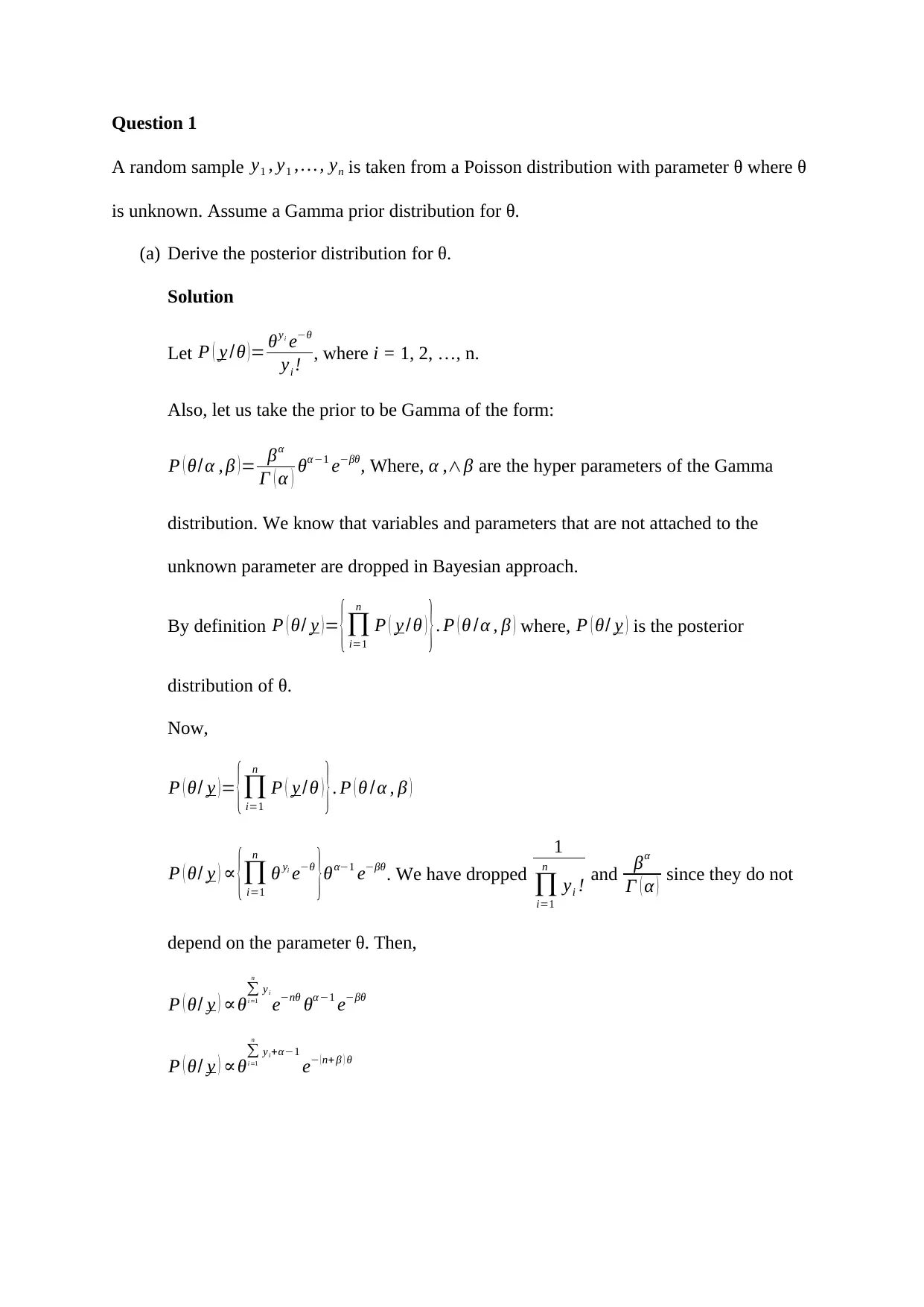
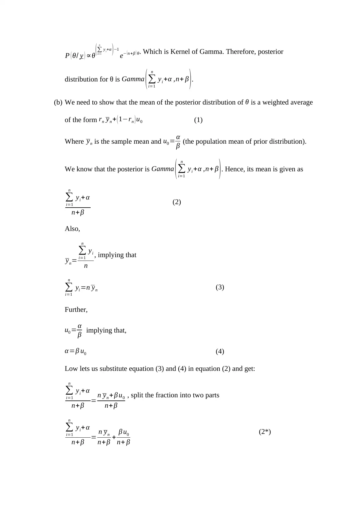
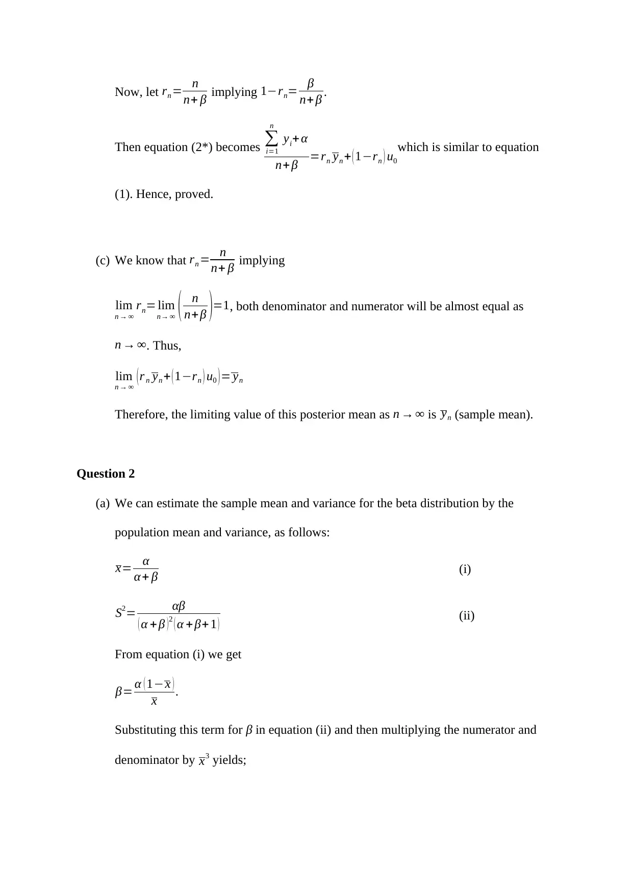
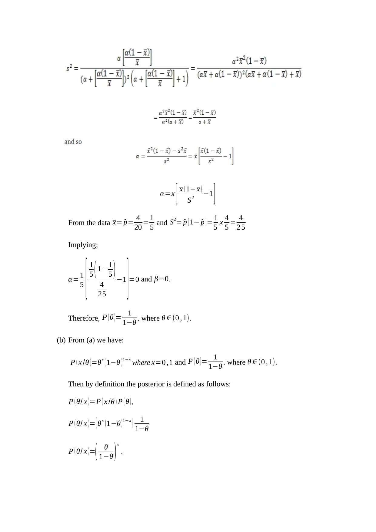
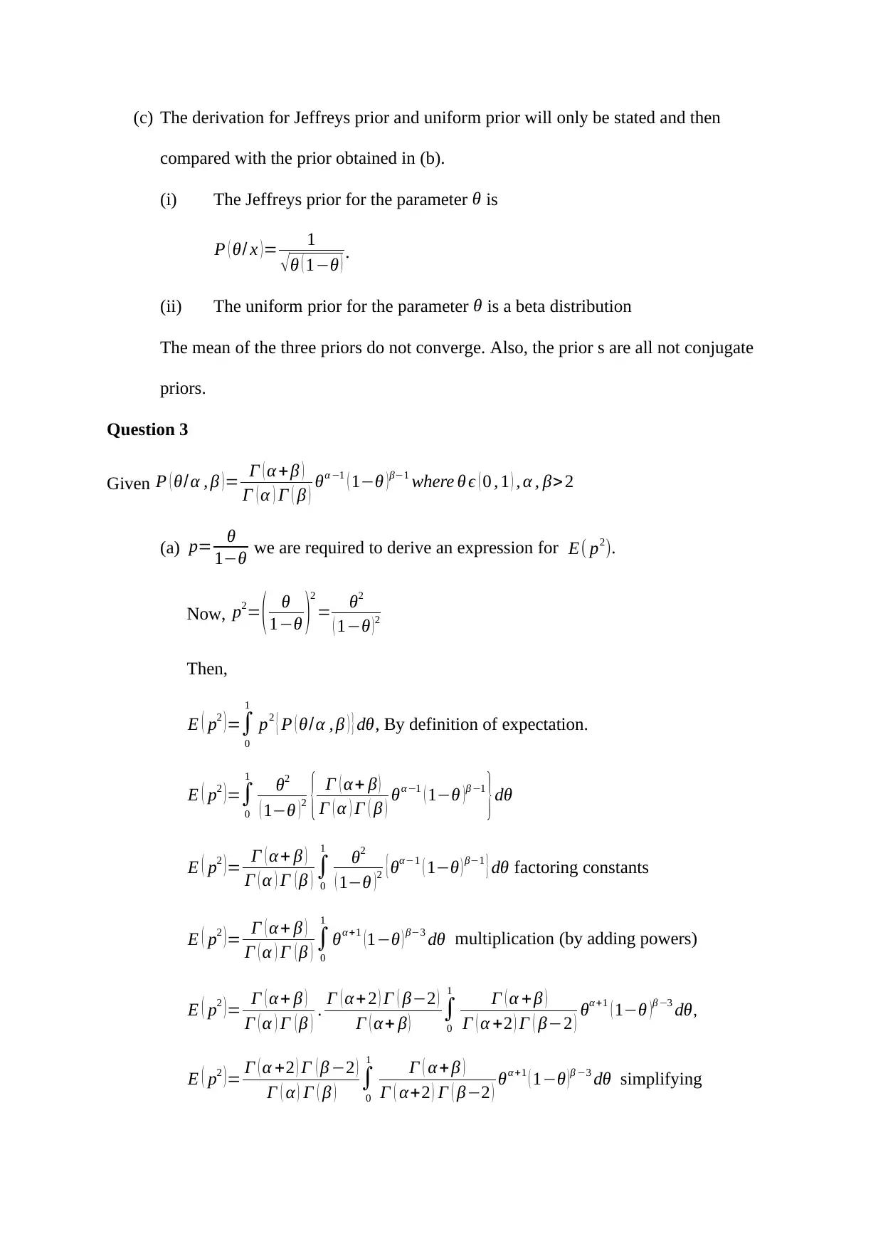
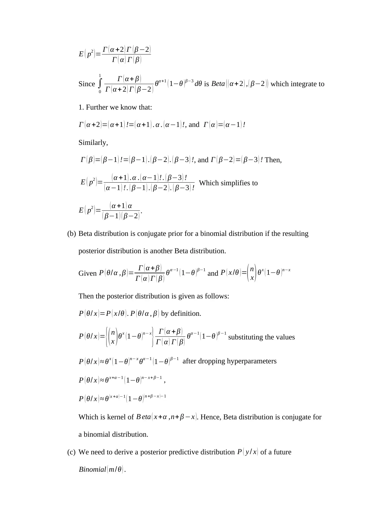
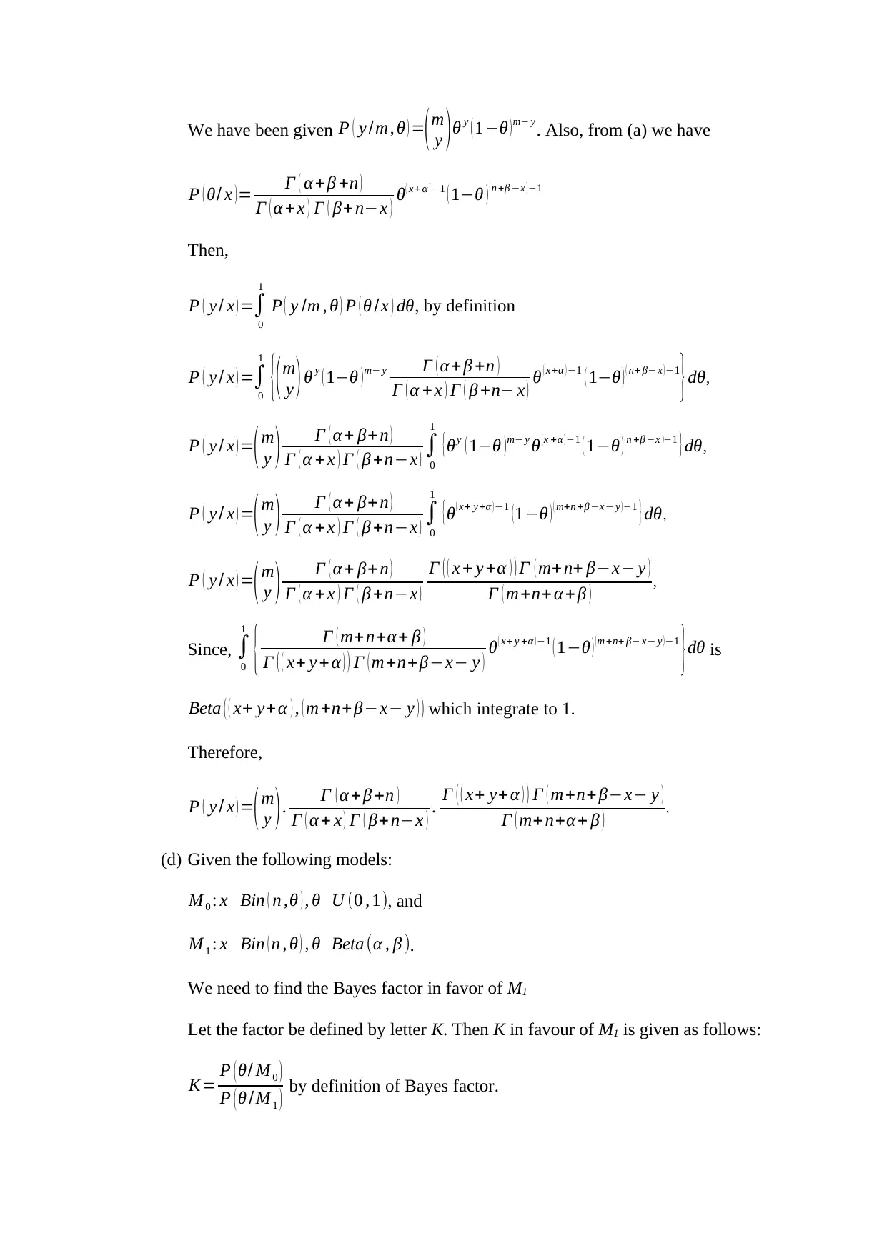
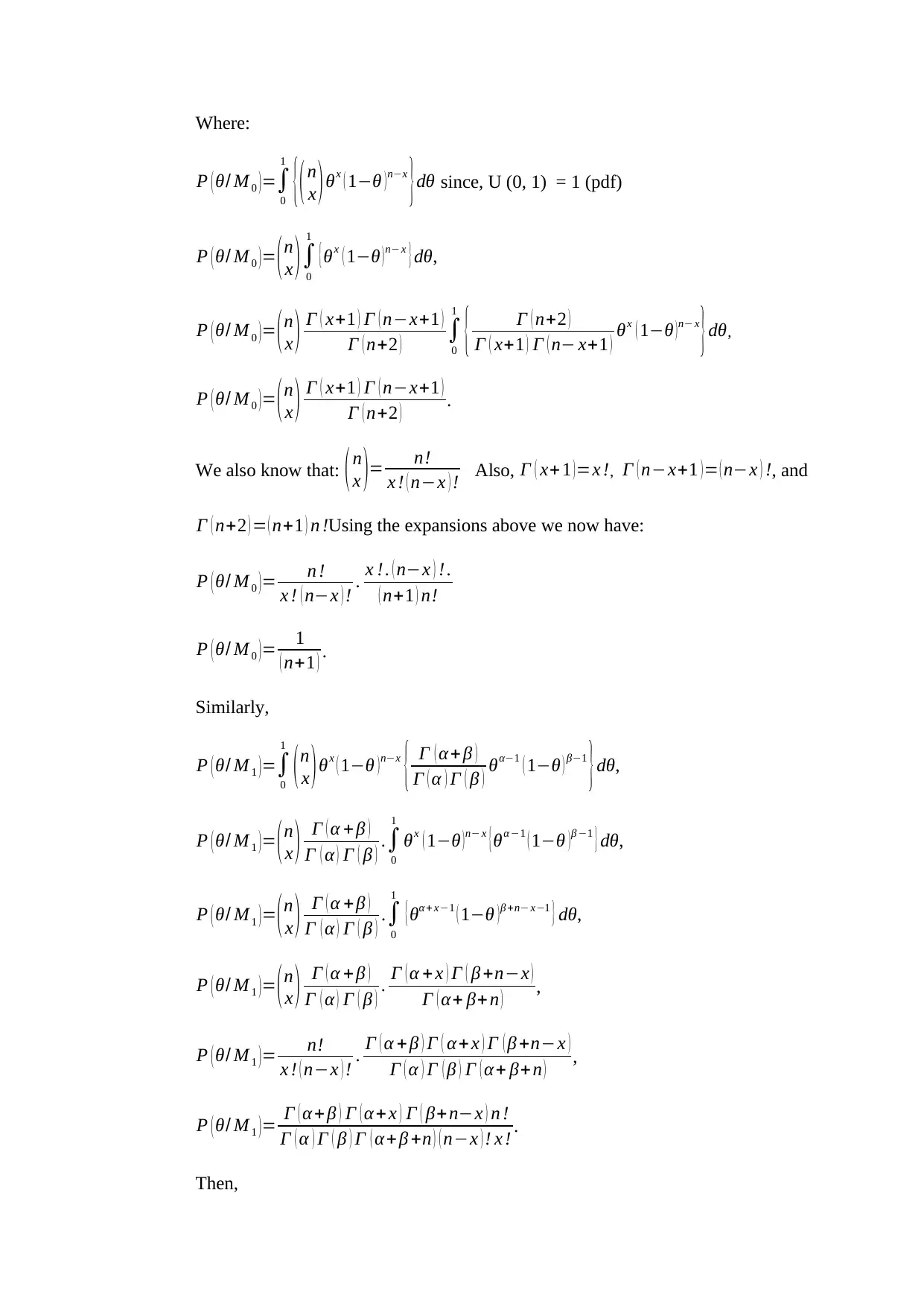
This assignment solution addresses key concepts in Bayesian inference, focusing on statistical distributions and their applications. It begins by deriving the posterior distribution for a Poisson distribution with a Gamma prior and demonstrates how the mean of the posterior distribution is a weighted average of the sample mean and the prior mean. The solution then delves into estimating sample mean and variance for a Beta distribution using the method of moments, deriving the corresponding posterior distribution. The assignment further explores the derivation of expectations and the concept of conjugate priors within the context of binomial distributions. Finally, it calculates the posterior predictive distribution and determines the Bayes factor for comparing different models. The solutions provide detailed derivations and explanations for each step, making it a valuable resource for students studying Bayesian inference.

Question 1
A random sample y1 , y1 , … , yn is taken from a Poisson distribution with parameter θ where θ
is unknown. Assume a Gamma prior distribution for θ.
(a) Derive the posterior distribution for θ.
Solution
Let P ( y /θ ) = θyi
e−θ
yi ! , where i = 1, 2, …, n.
Also, let us take the prior to be Gamma of the form:
P ( θ/α , β ) = βα
Γ ( α ) θα −1 e−βθ, Where, α ,∧β are the hyper parameters of the Gamma
distribution. We know that variables and parameters that are not attached to the
unknown parameter are dropped in Bayesian approach.
By definition P ( θ/ y )= {∏
i=1
n
P ( y /θ ) }. P ( θ /α , β ) where, P ( θ/ y ) is the posterior
distribution of θ.
Now,
P ( θ/ y ) = {∏
i=1
n
P ( y /θ ) } . P ( θ /α , β )
P ( θ/ y ) ∝ {∏
i=1
n
θ yi
e−θ
}θα−1 e−βθ. We have dropped
1
∏
i=1
n
yi ! and βα
Γ ( α ) since they do not
depend on the parameter θ. Then,
P ( θ/ y ) ∝θ∑
i=1
n
yi
e−nθ θα−1 e−βθ
P ( θ/ y ) ∝θ∑
i=1
n
yi+α−1
e− ( n+ β ) θ

P ( θ/ y ) ∝θ (∑
i=1
n
yi+α )−1
e− (n +β ) θ. Which is Kernel of Gamma. Therefore, posterior
distribution for θ is Gamma ( ∑
i=1
n
yi +α ,n+ β ).
(b) We need to show that the mean of the posterior distribution of θ is a weighted average
of the form rn yn + ( 1−rn ) u0 (1)
Where yn is the sample mean and u0 = α
β (the population mean of prior distribution).
We know that the posterior is Gamma ( ∑
i=1
n
yi +α ,n+ β ). Hence, its mean is given as
∑
i=1
n
yi+ α
n+β
(2)
Also,
yn=
∑
i=1
n
yi
n
, implying that
∑
i=1
n
yi =n yn (3)
Further,
u0 = α
β implying that,
α =β u0 (4)
Low lets us substitute equation (3) and (4) in equation (2) and get:
∑
i=1
n
yi+ α
n+β = n yn + β u0
n+ β
, split the fraction into two parts
∑
i=1
n
yi+α
n+ β = n yn
n+β + β u0
n+ β
(2*)

Now, let rn = n
n+ β implying 1−rn= β
n+ β .
Then equation (2*) becomes ∑
i=1
n
yi+ α
n+ β =rn yn + ( 1−rn ) u0
which is similar to equation
(1). Hence, proved.
(c) We know that rn = n
n+ β implying
lim
n → ∞
rn= lim
n→ ∞ ( n
n+β )=1, both denominator and numerator will be almost equal as
n → ∞. Thus,
lim
n → ∞ ( r n yn + ( 1−rn ) u0 ) = yn
Therefore, the limiting value of this posterior mean as n → ∞ is yn (sample mean).
Question 2
(a) We can estimate the sample mean and variance for the beta distribution by the
population mean and variance, as follows:
x= α
α + β (i)
S2= αβ
( α +β )2 ( α +β+1 ) (ii)
From equation (i) we get
β= α ( 1−x )
x .
Substituting this term for β in equation (ii) and then multiplying the numerator and
denominator by x3 yields;

α =x [ x ( 1−x )
S2 −1 ]
From the data x= ^p= 4
20 = 1
5 and S2= ^p ( 1− ^p )= 1
5 x 4
5 = 4
2 5
Implying;
α = 1
5 [ 1
5 (1− 1
5 )
4
25
−1
]=0 and β=0.
Therefore, P ( θ )= 1
1−θ . where θ ∈(0 , 1).
(b) From (a) we have:
P ( x /θ ) =θx ( 1−θ ) 1−x where x=0 ,1 and P ( θ )= 1
1−θ . where θ ∈(0 , 1).
Then by definition the posterior is defined as follows:
P ( θ/ x ) =P ( x /θ ) P ( θ ),
P ( θ/ x )= {θx (1−θ )1− x } 1
1−θ
P ( θ/ x ) =( θ
1−θ ) x
.

(c) The derivation for Jeffreys prior and uniform prior will only be stated and then
compared with the prior obtained in (b).
(i) The Jeffreys prior for the parameter θ is
P ( θ/ x )= 1
√θ ( 1−θ ) .
(ii) The uniform prior for the parameter θ is a beta distribution
The mean of the three priors do not converge. Also, the prior s are all not conjugate
priors.
Question 3
Given P ( θ/α , β )= Γ ( α +β )
Γ ( α ) Γ ( β ) θα −1 ( 1−θ )β−1 where θ ϵ ( 0 , 1 ) , α , β>2
(a) p= θ
1−θ we are required to derive an expression for E( p2).
Now, p2= ( θ
1−θ )
2
= θ2
( 1−θ ) 2
Then,
E ( p2 ) =∫
0
1
p2 { P ( θ/α , β ) } dθ, By definition of expectation.
E ( p2 ) =∫
0
1
θ2
( 1−θ ) 2 { Γ ( α+ β )
Γ ( α ) Γ ( β ) θα−1 ( 1−θ ) β −1
} dθ
E ( p2 )= Γ ( α + β )
Γ ( α ) Γ ( β ) ∫
0
1
θ2
( 1−θ )2 {θα−1 ( 1−θ ) β−1 } dθ factoring constants
E ( p2 ) = Γ ( α + β )
Γ ( α ) Γ ( β ) ∫
0
1
θα +1 ( 1−θ ) β−3 dθ multiplication (by adding powers)
E ( p2 )= Γ ( α + β )
Γ ( α ) Γ ( β ) . Γ ( α + 2 ) Γ ( β−2 )
Γ ( α + β ) ∫
0
1 Γ ( α +β )
Γ ( α +2 ) Γ ( β−2 ) θα+1 ( 1−θ )β −3 dθ,
E ( p2 )= Γ ( α +2 ) Γ ( β −2 )
Γ ( α ) Γ ( β ) ∫
0
1 Γ ( α+ β )
Γ ( α+2 ) Γ ( β−2 ) θα+1 ( 1−θ )β −3 dθ simplifying

E ( p2 )= Γ ( α +2 ) Γ ( β −2 )
Γ ( α ) Γ ( β )
Since ∫
0
1 Γ ( α + β )
Γ ( α + 2 ) Γ ( β−2 ) θα +1 ( 1−θ ) β−3 dθ is Beta ( ( α + 2 ) , ( β−2 ) ) which integrate to
1. Further we know that:
Γ ( α +2 )= ( α +1 ) != ( α +1 ) . α . ( α −1 ) !, and Γ ( α )= ( α−1 ) !
Similarly,
Γ ( β )= ( β−1 ) != ( β−1 ) . ( β−2 ) . ( β−3 ) !, and Γ ( β−2 ) = ( β−3 ) ! Then,
E ( p2 )= ( α +1 ) .α . ( α−1 ) ! . ( β−3 ) !
( α −1 ) !. ( β−1 ) . ( β−2 ) . ( β−3 ) ! Which simplifies to
E ( p2 )= ( α +1 ) α
( β−1 ) ( β−2 ) .
(b) Beta distribution is conjugate prior for a binomial distribution if the resulting
posterior distribution is another Beta distribution.
Given P ( θ/α , β )= Γ ( α +β )
Γ ( α ) Γ ( β ) θα −1 ( 1−θ )β−1 and P ( x /θ ) =( n
x ) θx ( 1−θ ) n−x
Then the posterior distribution is given as follows:
P ( θ/ x ) =P ( x /θ ) . P ( θ/α , β ) by definition.
P ( θ/ x ) = {( n
x ) θx ( 1−θ ) n− x
} Γ ( α + β )
Γ ( α ) Γ ( β ) θα −1 ( 1−θ ) β −1
substituting the values
P ( θ/ x ) ≈ θx ( 1−θ )n− x θα−1 (1−θ ) β−1 after dropping hyperparameters
P ( θ/ x ) ≈ θx+α −1 ( 1−θ ) n− x+ β−1 ,
P ( θ/ x ) ≈ θ ( x +α ) −1 ( 1−θ ) ( n +β −x )−1
Which is kernel of B eta ( x +α ,n+ β −x ). Hence, Beta distribution is conjugate for
a binomial distribution.
(c) We need to derive a posterior predictive distribution P ( y / x ) of a future
Binomial ( m/θ ) .

We have been given P ( y /m, θ ) =( m
y ) θ y ( 1−θ ) m− y
. Also, from (a) we have
P ( θ/ x )= Γ ( α+ β +n )
Γ ( α +x ) Γ ( β+ n−x ) θ ( x+ α )−1 ( 1−θ ) (n +β −x )−1
Then,
P ( y / x ) =∫
0
1
P ( y /m , θ ) P ( θ /x ) dθ, by definition
P ( y / x ) =∫
0
1
{(m
y )θ y ( 1−θ )m− y Γ ( α+β +n )
Γ ( α + x ) Γ ( β +n− x ) θ ( x+α )−1 ( 1−θ ) ( n+ β− x )−1
}dθ,
P ( y / x ) =(m
y ) Γ ( α+ β+n )
Γ ( α + x ) Γ ( β +n−x ) ∫
0
1
{θy ( 1−θ )m− y θ (x +α )−1 ( 1−θ ) (n +β −x )−1 } dθ,
P ( y / x ) =(m
y ) Γ ( α+ β+n )
Γ ( α + x ) Γ ( β +n−x ) ∫
0
1
{θ ( x+ y+α )−1 (1−θ ) ( m+n +β −x− y )−1 } dθ,
P ( y / x ) =
(m
y ) Γ ( α+ β+n )
Γ ( α + x ) Γ ( β +n−x )
Γ ( ( x + y +α ) ) Γ ( m+ n+ β−x− y )
Γ ( m+n+ α + β ) ,
Since, ∫
0
1
{ Γ ( m+ n+α+ β )
Γ ( ( x+ y + α ) ) Γ ( m+n+ β−x− y ) θ ( x+ y +α )−1 ( 1−θ ) (m +n+ β− x− y )−1
}dθ is
Beta ( ( x+ y+α ) , ( m+n+ β−x− y ) ) which integrate to 1.
Therefore,
P ( y / x ) =(m
y ). Γ ( α + β +n )
Γ ( α+ x ) Γ ( β+ n−x ) . Γ ( ( x+ y+ α ) ) Γ ( m+n+ β−x− y )
Γ ( m+ n+α + β ) .
(d) Given the following models:
M 0 : x Bin ( n ,θ ) , θ U (0 , 1), and
M 1 : x Bin ( n , θ ) , θ Beta (α , β ).
We need to find the Bayes factor in favor of M1
Let the factor be defined by letter K. Then K in favour of M1 is given as follows:
K= P ( θ/ M0 )
P ( θ / M1 ) by definition of Bayes factor.

Where:
P ( θ/ M 0 )=∫
0
1
{(n
x )θx ( 1−θ )n−x
}dθ since, U (0, 1) = 1 (pdf)
P ( θ/ M 0 )= ( n
x ) ∫
0
1
{ θx ( 1−θ ) n− x } dθ,
P ( θ/ M 0 )= ( n
x ) Γ ( x+1 ) Γ ( n−x+1 )
Γ ( n+2 ) ∫
0
1
{ Γ ( n+2 )
Γ ( x+1 ) Γ ( n− x+1 ) θx ( 1−θ ) n− x
} dθ,
P ( θ/ M 0 )= (n
x ) Γ ( x+1 ) Γ ( n−x+1 )
Γ ( n+2 ) .
We also know that: ( n
x )= n!
x ! ( n−x ) ! Also, Γ ( x+ 1 )=x !, Γ ( n−x+1 ) = ( n−x ) !, and
Γ ( n+2 ) = ( n+1 ) n !Using the expansions above we now have:
P ( θ/ M 0 )= n !
x ! ( n−x ) ! . x ! . ( n−x ) !.
( n+1 ) n!
P ( θ/ M 0 )= 1
( n+1 ) .
Similarly,
P ( θ/ M 1 )=∫
0
1
( n
x ) θx ( 1−θ ) n−x
{ Γ ( α+ β )
Γ ( α ) Γ ( β ) θα−1 ( 1−θ ) β−1
} dθ,
P ( θ/ M 1 )= ( n
x ) Γ ( α + β )
Γ ( α ) Γ ( β ) .∫
0
1
θx ( 1−θ ) n− x { θα−1 ( 1−θ ) β −1 } dθ,
P ( θ/ M1 ) = ( n
x ) Γ ( α +β )
Γ ( α ) Γ ( β ) .∫
0
1
{ θα+ x−1 ( 1−θ ) β +n− x−1 } dθ,
P ( θ/ M 1 )= ( n
x ) Γ ( α + β )
Γ ( α ) Γ ( β ) . Γ ( α + x ) Γ ( β +n−x )
Γ ( α+ β+ n ) ,
P ( θ/ M 1 )= n!
x ! ( n−x ) ! . Γ ( α + β ) Γ ( α + x ) Γ ( β +n−x )
Γ ( α ) Γ ( β ) Γ ( α+ β+n ) ,
P ( θ/ M 1 )= Γ ( α + β ) Γ ( α+ x ) Γ ( β+n−x ) n !
Γ ( α ) Γ ( β ) Γ ( α+β +n ) ( n−x ) ! x ! .
Then,

K= Γ ( α ) Γ ( β ) Γ ( α + β+ n ) ( n−x ) ! x !
(n+1) Γ ( α +β ) Γ ( α+ x ) Γ ( β +n−x ) n ! .