CEN4017: Risk Management in Projects Report, Teesside University

This report, prepared for a MSc Project Management course (CEN4017) at Teesside University, examines risk management in projects. It begins with a decision tree analysis for the ABC Computer Company, evaluating bidding strategies and manufacturing processes using Expected Monetary Value (EMV) and Bayer's Rule. The report then delves into an optimization model for the Pigskin Company, addressing production planning and cost minimization through sensitivity analysis and spreadsheet models. Finally, the report presents a linear programming problem for the GulfGolf Company, aiming to maximize profit by optimizing the production of golf bags, including graphical representations and solver solutions. The report adheres to strict formatting guidelines and includes references in Harvard style, demonstrating a comprehensive understanding of risk management principles and practical application in project scenarios.

Risk Management 1
RISK MANAGEMENT
Student Name
Course
Professor
University
City (State)
Date

Risk Management 2
Risk Management
Q.1 Decision Tree for ABC Computer Company
ABC is bidding at $9,500 per computer while Complex is tendering for $10,000. To
put this into context, if it wins the tender, ABC will generate in excess of $9 million in net
profit; with a net profit of $1,000,000 - 10,000 x $8,500 + 10,000 x $ 9,500 = $9,000,000. In
this decision tree, there are several decision nodes and in order to get the values correctly, the
bid amount is the first decision, followed by the manufacturing process, which also follows a
similar procedure as the previous calculation commonly applied for uncertain dependent
procedures (Zhou et al.,2018, p.1254).
Expected Monetary Value (EMV)
The calculation begins at the top right chance node of the tree and once the expected values
are obtained, ¼ x $9 + ½ x$19+ ¼ x $44 =$22.75. It implies that the top branch is the
preferred branch having a higher expected value while the bottom branch is to have a value of
$14. If the proposed manufacturing process is used, the value for the corresponding decision
node is equal to $22.75. Going back to the root of the decision tree, the leftmost chance
node’s value shall be 1/3 x $22.75 + 2/3 x -$1=$6.92. The expected values for the other three
branches will be calculated in a similar way and the results of the calculations indicate that
placing a bid at $8,500 will give the highest value at $8.17 million. ABC should then decide
on its bid price at $8,500 and also use the new manufacturing process if the tender is awarded
to them. The other branches which have been indicated on the decision tree with cross
hatching are less important (Keller, 2015 p.898)
Bayer’s Rule
In scenarios involving a decision tree with several stages, branches of probability on
the right side have restrictions to outcomes that have happened previously (Stone, 2016 p.8).

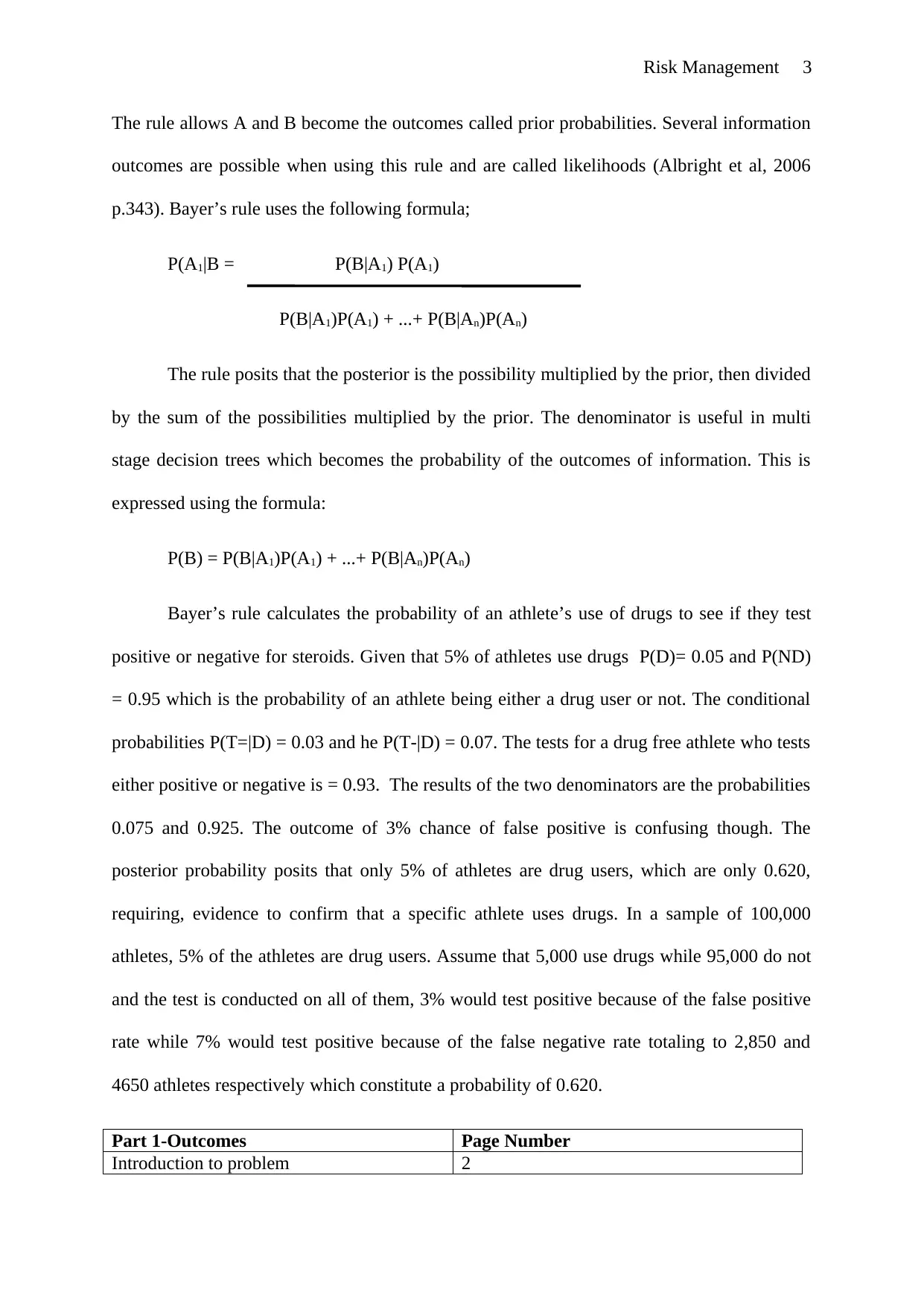
Risk Management 3
The rule allows A and B become the outcomes called prior probabilities. Several information
outcomes are possible when using this rule and are called likelihoods (Albright et al, 2006
p.343). Bayer’s rule uses the following formula;
P(A1|B = P(B|A1) P(A1)
P(B|A1)P(A1) + ...+ P(B|An)P(An)
The rule posits that the posterior is the possibility multiplied by the prior, then divided
by the sum of the possibilities multiplied by the prior. The denominator is useful in multi
stage decision trees which becomes the probability of the outcomes of information. This is
expressed using the formula:
P(B) = P(B|A1)P(A1) + ...+ P(B|An)P(An)
Bayer’s rule calculates the probability of an athlete’s use of drugs to see if they test
positive or negative for steroids. Given that 5% of athletes use drugs P(D)= 0.05 and P(ND)
= 0.95 which is the probability of an athlete being either a drug user or not. The conditional
probabilities P(T=|D) = 0.03 and he P(T-|D) = 0.07. The tests for a drug free athlete who tests
either positive or negative is = 0.93. The results of the two denominators are the probabilities
0.075 and 0.925. The outcome of 3% chance of false positive is confusing though. The
posterior probability posits that only 5% of athletes are drug users, which are only 0.620,
requiring, evidence to confirm that a specific athlete uses drugs. In a sample of 100,000
athletes, 5% of the athletes are drug users. Assume that 5,000 use drugs while 95,000 do not
and the test is conducted on all of them, 3% would test positive because of the false positive
rate while 7% would test positive because of the false negative rate totaling to 2,850 and
4650 athletes respectively which constitute a probability of 0.620.
Part 1-Outcomes Page Number
Introduction to problem 2

Risk Management 4
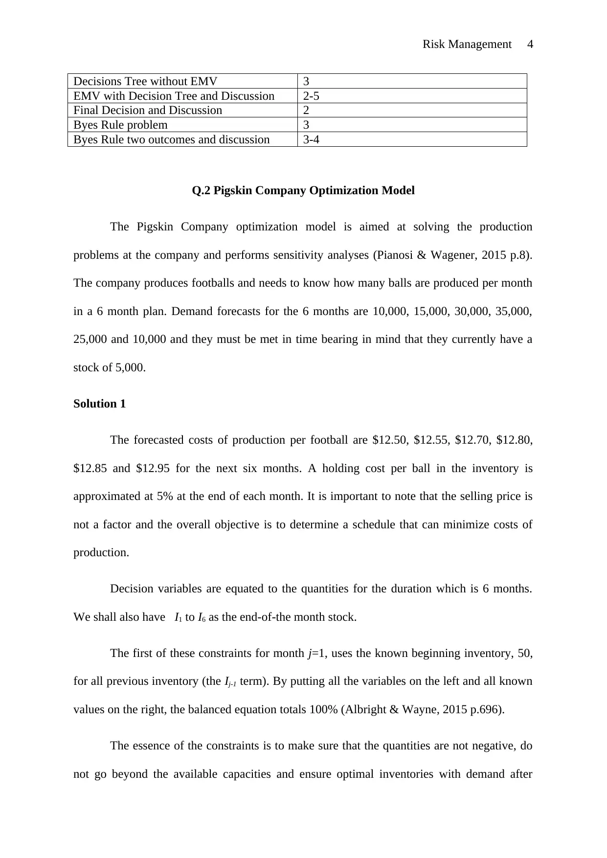
Decisions Tree without EMV 3
EMV with Decision Tree and Discussion 2-5
Final Decision and Discussion 2
Byes Rule problem 3
Byes Rule two outcomes and discussion 3-4
Q.2 Pigskin Company Optimization Model
The Pigskin Company optimization model is aimed at solving the production
problems at the company and performs sensitivity analyses (Pianosi & Wagener, 2015 p.8).
The company produces footballs and needs to know how many balls are produced per month
in a 6 month plan. Demand forecasts for the 6 months are 10,000, 15,000, 30,000, 35,000,
25,000 and 10,000 and they must be met in time bearing in mind that they currently have a
stock of 5,000.
Solution 1
The forecasted costs of production per football are $12.50, $12.55, $12.70, $12.80,
$12.85 and $12.95 for the next six months. A holding cost per ball in the inventory is
approximated at 5% at the end of each month. It is important to note that the selling price is
not a factor and the overall objective is to determine a schedule that can minimize costs of
production.
Decision variables are equated to the quantities for the duration which is 6 months.
We shall also have I1 to I6 as the end-of-the month stock.
The first of these constraints for month j=1, uses the known beginning inventory, 50,
for all previous inventory (the Ij-1 term). By putting all the variables on the left and all known
values on the right, the balanced equation totals 100% (Albright & Wayne, 2015 p.696).
The essence of the constraints is to make sure that the quantities are not negative, do
not go beyond the available capacities and ensure optimal inventories with demand after

Risk Management 5
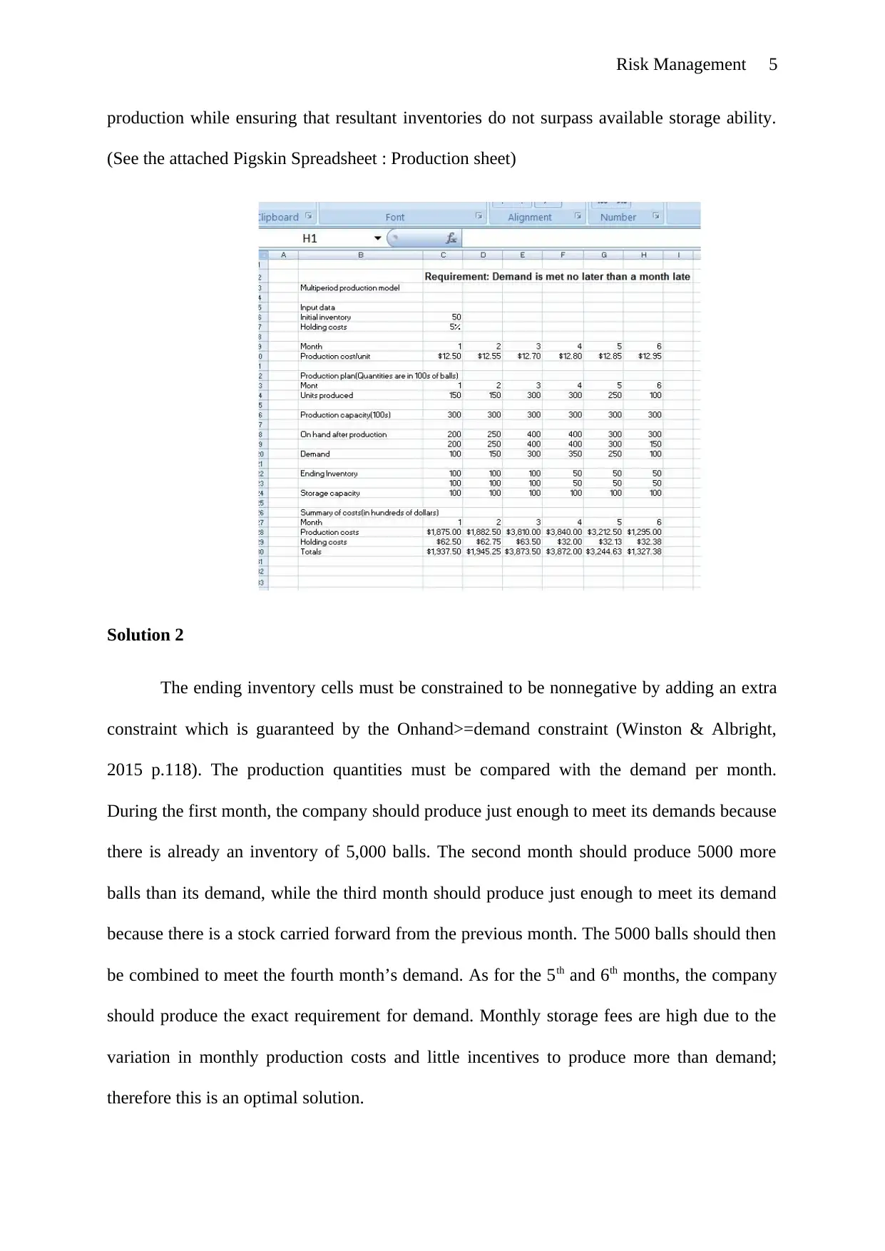
production while ensuring that resultant inventories do not surpass available storage ability.
(See the attached Pigskin Spreadsheet : Production sheet)
Solution 2
The ending inventory cells must be constrained to be nonnegative by adding an extra
constraint which is guaranteed by the Onhand>=demand constraint (Winston & Albright,
2015 p.118). The production quantities must be compared with the demand per month.
During the first month, the company should produce just enough to meet its demands because
there is already an inventory of 5,000 balls. The second month should produce 5000 more
balls than its demand, while the third month should produce just enough to meet its demand
because there is a stock carried forward from the previous month. The 5000 balls should then
be combined to meet the fourth month’s demand. As for the 5th and 6th months, the company
should produce the exact requirement for demand. Monthly storage fees are high due to the
variation in monthly production costs and little incentives to produce more than demand;
therefore this is an optimal solution.

Risk Management 6
(See the attached Pigskin Spreadsheet : Optimal model)
Solution 3
A sensitivity analysis is required because we know the inventory contains 5000
footballs although the storage capacity is 10,000 balls. Partly this is prohibitive because of the
5% holding fee and a modification to the previous spreadsheet to track the maximum ending
inventory is necessary. There are two possible scenarios; first, the percentage cost only
increases when the holding inventory increases and it is constant and second, optimal
production schedules impact on the outputs. There must be optimal production levels for each
month in a rolling planning horizon and therefore assumed demand whether real or forecast at
the end of scheduling will not affect optimal production.
(See the attached Pigskin Spreadsheet : Sensitivity Analysis)

Risk Management 7
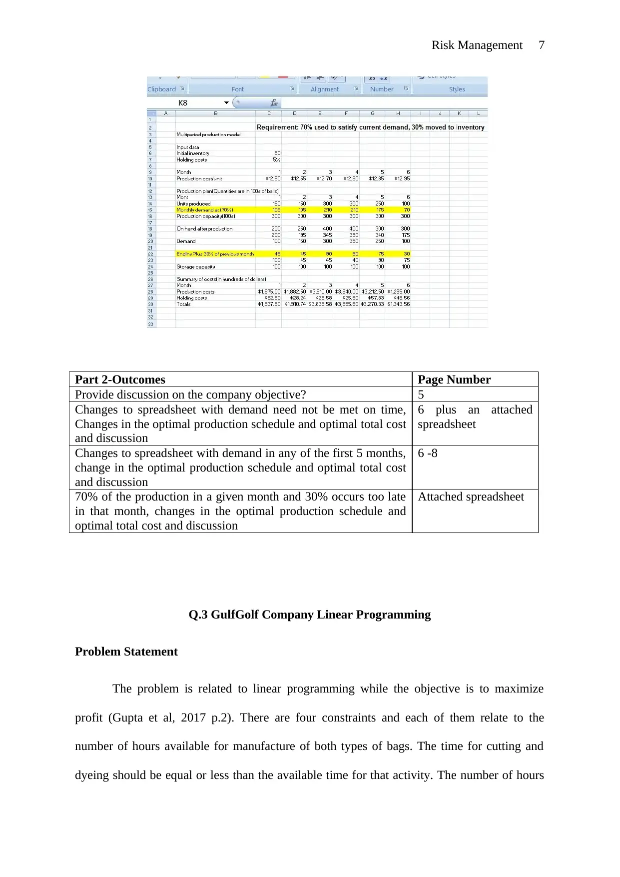
Part 2-Outcomes Page Number
Provide discussion on the company objective? 5
Changes to spreadsheet with demand need not be met on time,
Changes in the optimal production schedule and optimal total cost
and discussion
6 plus an attached
spreadsheet
Changes to spreadsheet with demand in any of the first 5 months,
change in the optimal production schedule and optimal total cost
and discussion
6 -8
70% of the production in a given month and 30% occurs too late
in that month, changes in the optimal production schedule and
optimal total cost and discussion
Attached spreadsheet
Q.3 GulfGolf Company Linear Programming
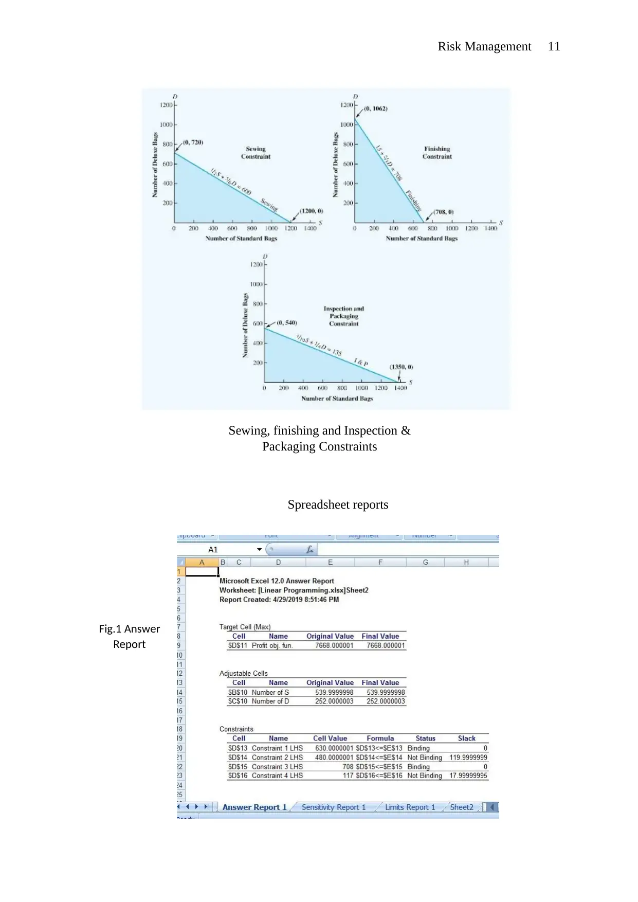
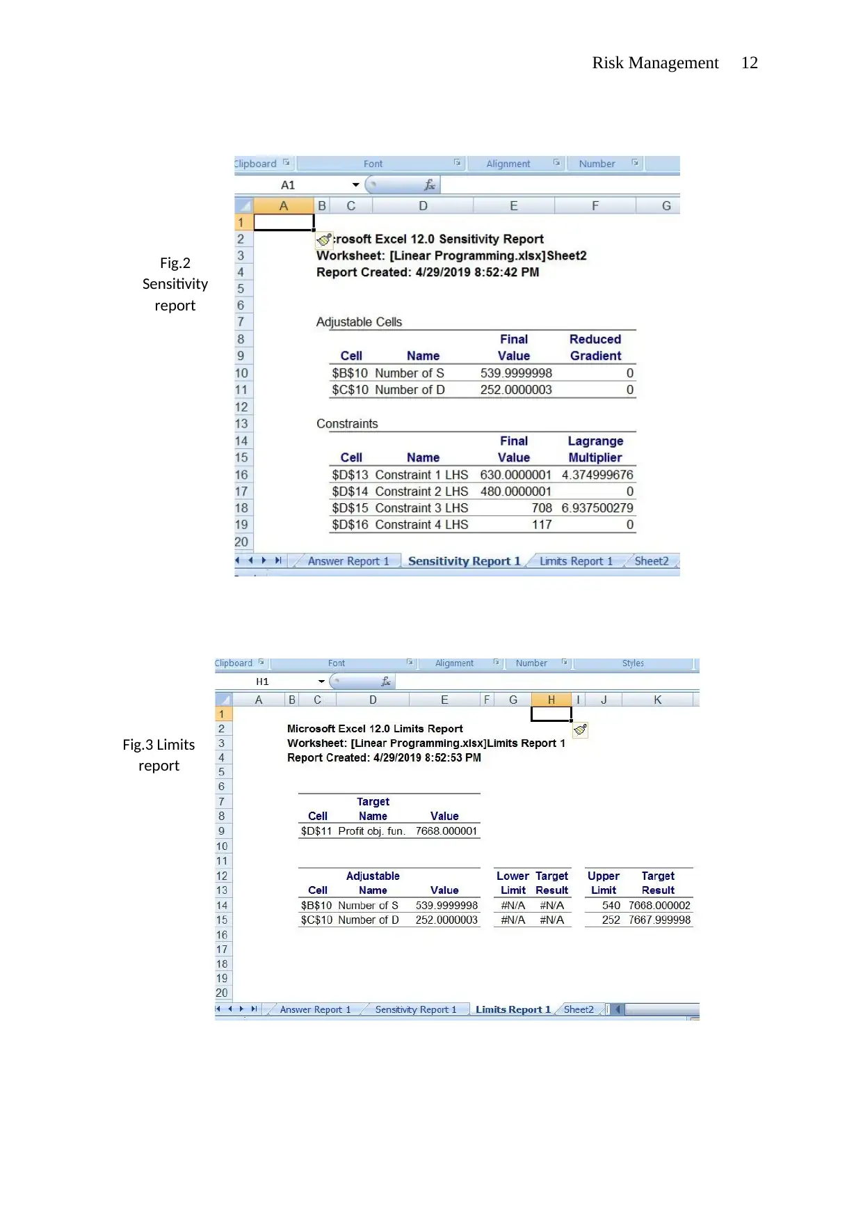
Problem Statement
The problem is related to linear programming while the objective is to maximize
profit (Gupta et al, 2017 p.2). There are four constraints and each of them relate to the
number of hours available for manufacture of both types of bags. The time for cutting and
dyeing should be equal or less than the available time for that activity. The number of hours

Risk Management 8
used for sewing must be less than or equal to the availed time for the activity. The number of
hours used for finishing must be equal or less than the duration allocated for that activity and
so is the case for inspection and packaging.
Discussion
A mathematical model of the problem at the company can be used to determine the
number of bags to produce in order to maximize profitability. Translating these verbal
statements into a mathematical is called problem formulation (Anderson et al., 2018, p.33).
Problems have unique features and in model formulation, guidelines such as fully
understanding the problem, describing the objective clearly, describe the objectives and each
constraint as well as define the decision variables.
The decision variables are determined after identifying the constraints where the
controllable inputs are the production of standard bags and deluxe bags. The decision
variables therefore will be S = number of standard bags and D = number of deluxe bags.
Now using the decision variables it is easy to write the objectives of the company.
The two sources of revenue for the company are the manufacture of standard bags (S) and
deluxe bags (D). if it sells a standard bag at $10, the company makes $10s and if it sells
deluxe bags at $9, it makes $9D, hence the total profit will be calculated as: Total profit =
10S + 9D. Maximizing profit is the objective of the decision variables S and D, and therefore
10S+9D is called an objective function. The objective is therefore Max 10S+9D.
After this the constraints must be expressed with reference to the decision variables
(Ploskas & Samaras, 2017 p.14). Constraint 1 is expressed as (Hours of cutting and dyeing) ≤
(Hours of cutting and dyeing time available). The above formula implies that each standard
bag produced will use 7/10 hours cutting and dyeing and therefore the number of hours taken
is 7/10S while a deluxe bag will use 1 hour thus deluxe bags will use 1D hours. Cutting and

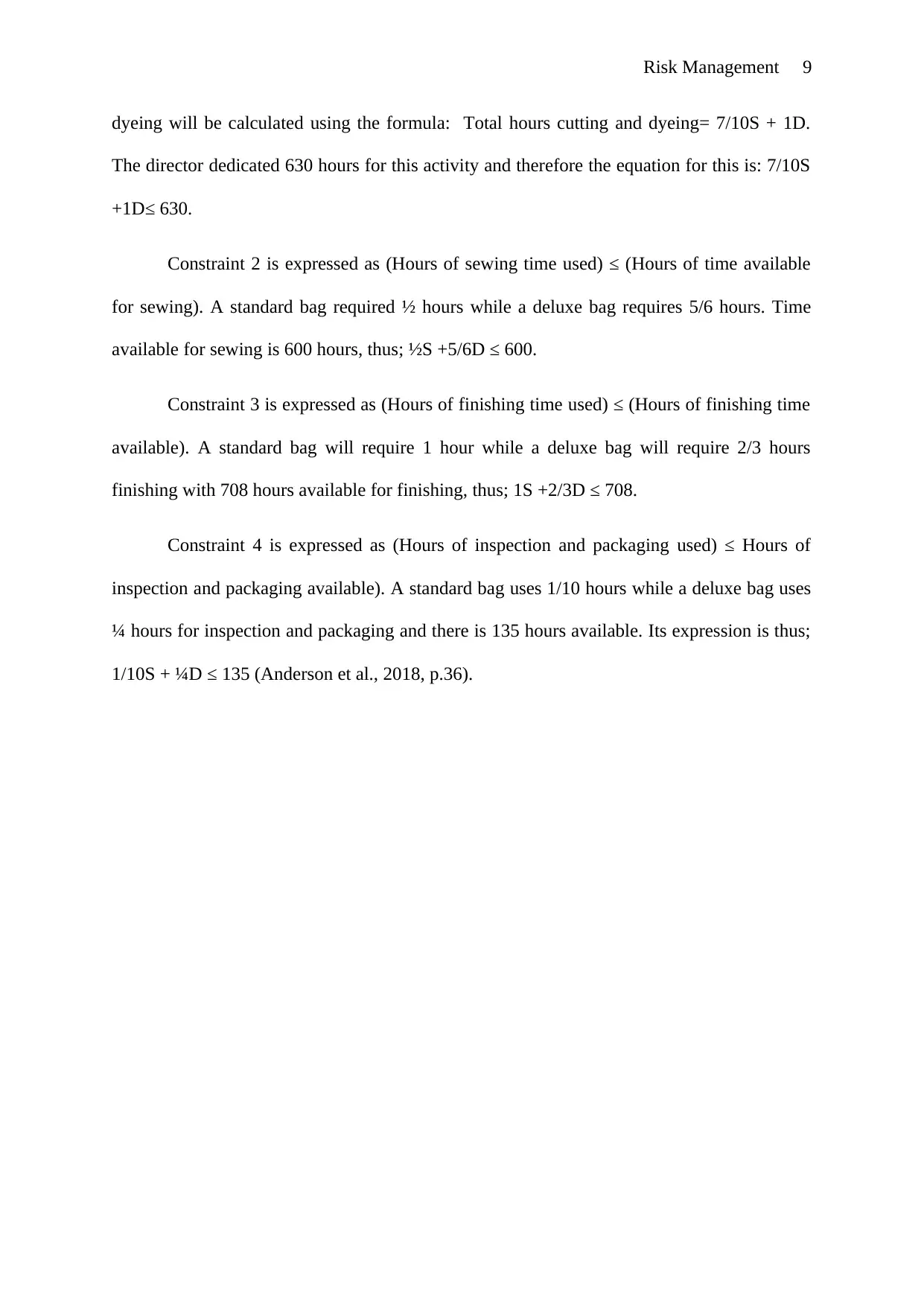
Risk Management 9
dyeing will be calculated using the formula: Total hours cutting and dyeing= 7/10S + 1D.
The director dedicated 630 hours for this activity and therefore the equation for this is: 7/10S
+1D≤ 630.
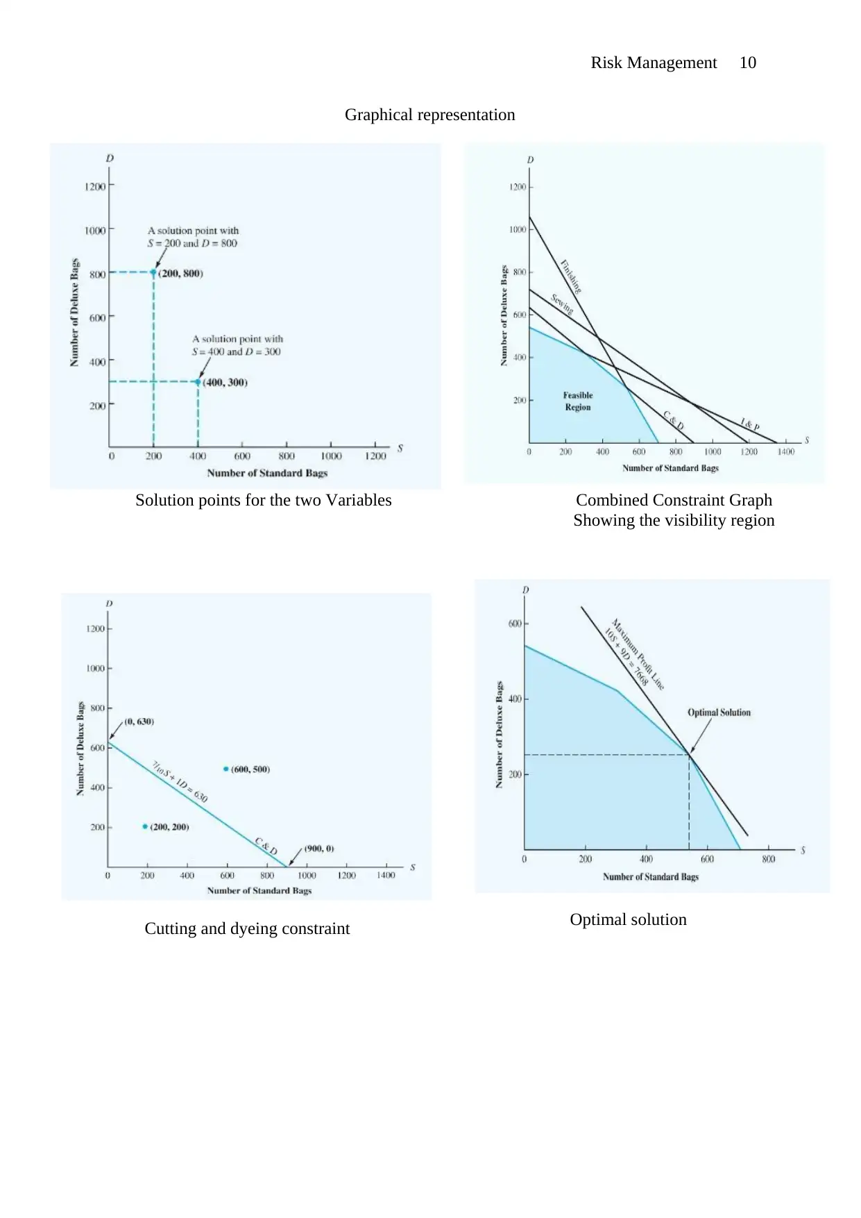
Constraint 2 is expressed as (Hours of sewing time used) ≤ (Hours of time available
for sewing). A standard bag required ½ hours while a deluxe bag requires 5/6 hours. Time
available for sewing is 600 hours, thus; ½S +5/6D ≤ 600.
Constraint 3 is expressed as (Hours of finishing time used) ≤ (Hours of finishing time
available). A standard bag will require 1 hour while a deluxe bag will require 2/3 hours
finishing with 708 hours available for finishing, thus; 1S +2/3D ≤ 708.
Constraint 4 is expressed as (Hours of inspection and packaging used) ≤ Hours of
inspection and packaging available). A standard bag uses 1/10 hours while a deluxe bag uses
¼ hours for inspection and packaging and there is 135 hours available. Its expression is thus;
1/10S + ¼D ≤ 135 (Anderson et al., 2018, p.36).

Combined Constraint Graph
Showing the visibility region
Solution points for the two Variables
Cutting and dyeing constraint Optimal solution
Risk Management 10
Graphical representation

Risk Management 11
Spreadsheet reports
Sewing, finishing and Inspection &
Packaging Constraints
Fig.1 Answer
Report

Risk Management 12
Fig.2
Sensitivity
report
Fig.3 Limits
report

Risk Management 13
Part 3-Outcomes Page Number
Problem statement 9
Discussion data, constraints type and objectives 9
Analytical equations with condition forms 10
Co-ordinates for graphs, Graphical representation,
Feasible region hatching
11-13
Final number for standard and deluxe bag and discussion
Spread sheet model and solver solution Attached excel workbook
Question 4: Network diagrams and time estimates
Start
A
B
C
D
G
E
I
HF J
K
FinishL M N
O
P
Q
R
Figure 1: Network Diagram for the project
On the network diagram, there consists of 18 tasks named from A to R. The tasks are
based on software development processes, with the optimistic, pessimistic and most likely
durations well presented in the chart for the sake of analysis (Taherdoost, H., &
Keshavarzsaleh, 2018).
Table 1:Project estimates
Time Estimates for
Reliable’s Project
Activity Time o
+4m+p
A
ctivity
Mean
(μ)
Ac
tivity
Variance
O
(optimistic)
M
(most
likely)
P
(pessimistic
)
A 1 2 3 1
2
2 0.1
1
B 1 2 3 1
2
2 0.1
1
C 0.5 1 1.5 6 1 0.0
3

Risk Management 14
D 0.5 1 1.5 6 1 0.0
3
E 3 4 5 2
4
4 0.1
1
F 1 2 3 1
2
2 0.1
1
G 3 5 7 3
0
5 0.4
4
H 1 2 3 1
2
2 0.1
1
I 10 1
2
14 7
2
1
2
0.4
4
J 1 2 3 1
2
2 0.1
1
K 0.5 1 1.5 6 1 0.0
3
L 0.5 1 1.5 6 1 0.0
3
M 4 6 8 3
6
6 0.4
4
N 0.5 1 1.5 6 1 0.0
3
O 1 2 3 1
2
2 0.1
1
P 1.5 3 4.5 1
8
3 0.2
5
Q 1 2 3 1
2
2 0.1
1
R 2 4 6 2
4
4 0.4
4
On the calculations, the expected activity times are shown as 2 weeks for tasks A,B,
F, J,O and Q. Tasks C,D,K,L and M are expected to take a period one week towards
completion. Task P is expected to take 3 weeks, tasks E and R taking a period of 4 weeks
each, task M taking 6 weeks as task I taking a period of 12 weeks to completion, probably the
highest expected completion times.
Table 2: Project times
Project time : 22
Mean = 26
Variance = 1.06
Standard
deviation = 1.03
d = 40

Risk Management 15
The project indicates an average of 26 weeks, with a variance of 1.06.
Table 3: Probabilities of completion
Finding prob.
Using excel
P(T<=44) = 1.0000
= 100.00%
At 44 weeks, the project will be complete. This indicates a probability of 0 that the
project lasts for 46 weeks. For 85% completion, the project will require 44 weeks to ensure
that portion completed.
The risk exposure will be measured using the times to completion and the quality of
software designed. The variations between the two (design risks) will be an indication of
some amounts of risk within the project.
Question 5 Risk Management
Project Network structure
Start
A
B
D E FinishC
Figure 2: Network diagram for the construction assignment

Risk Management 16
On the chart, the intermediaries between the different tasks within the construction
industry were stipulated within the given time limits. The tasks were four, defined as A,B,C
D and E, within the stipulated timelines.
Risk methodologies discussed
Table 4: Simulation of expected project times
Time Estimates for
Reliable’s Project
Activity
Time
o
+4m+
p
Acti
vity Mean
(μ)
A
ctivity
Varian
ce
O
(optimisti
c)
M
(mo
st
likel
y)
P
(pessimisti
c)
A 5 2 3 1
6.00 2.67
0
.11
B 10 2 3 2
1.00 3.50
1
.36
C 15 1 1.5 2
0.50 3.42
5
.06
D 5 1 1.5 1
0.50 1.75
0
.34
E 4 4 5 2
5.00 4.17
0
.03
On the activities, the maximum activity time had an average of 4.17 on activity E
followed by project B on the same averages. The activities A,C and D showed lower weeks
spent on each of the tasks.
Table 5: Summary statistics of the project times
Project time : 4
Mean = 9
Variance =
9
.00
Standard
deviation =
0
.05
d =
4
0

Risk Management 17
On the construction project, the average time is expected as 40 weeks with a standard
deviation of 0.05 weeks. The average time is 9 weeks for each of the individual task assigned
within the indicated project timelines. The risk methodology adopted in the plan is based on
quality well-crafted designs to cater for the challenges associated with design risks within the
construction activities.
Comparison of the results with the paper
In comparison with the paper, the analysis results in lower risks in terms of the
standard deviation realized at 0.05. The implication of the figure is that there exists less risks
within the construction activities in question 2 as opposed to the software development in the
first task.
In comparison to the table above, most of the risk factors within the construction
activities had higher standard deviations at 0.21. This implicates essence of risk management
for the entire activities within the entire project.
Effects of weather risk modelling using uniform distribution
Application of uniform distribution on weather results in lower levels of risk. The
approach lead to an indication of lower levels of uncertainty in terms of the extent of risk
realized over time.

Risk Management 18
Sensitivity analysis of the influence of the risk on the project outcomes
Sensitivity analysis is an important aspect of projects, owing to the fact that they
influence the quality and value of the project yields. The analysis is based on the levels of
risk, higher and lower risks in terms of the various activities involved (Yu, M., Zhu, F., Yang,
X., Wang, L., & Sun, 2018 p.784.). The outcome of the analysis helps project managers
come up with appropriate plans towards mitigation of risks within individual projects.
Part 5-Outcome Page Number
Excel model with description, Network Diagram with all values Q.5 spreadsheet
Simulation model with all the tables and probabilities,
descriptions provided with @RISK inputs and outputs
Q.5 spreadsheet
Result comparison discussion with paper, results representation
and analysis
17
Change in distribution, Uniform distribution and effect on
project duration and distribution properties discussion
17
Sensitivity analysis with discussion 18

Risk Management 19
Reference List
Albright, S.C. and Wayne, L., 2015. Winston. Business Analytics: Data Analysis and
Decision Making. Cengage Learning.–2014.–1008 p.
Anderson, D.R., Sweeney, D.J., Williams, T.A., Camm, J.D. and Cochran, J.J., 2018. An
introduction to management science: quantitative approach. Cengage learning.
Camm, J., Cochran, J., Fry, M., Ohlmann, J., Anderson, D., Sweeney, D. and Williams, T.
(n.d.). Quantitative Studies.
Dawood, N., 1998. Estimating project and activity duration: a risk management approach
using network analysis. Construction Management & Economics, 16(1), pp.41-48.
Gupta, A.D., Bokde, N., Marathe, D. and Kulat, K., 2017. Optimization techniques for
leakage management in urban water distribution networks. Water Science and
Technology: Water Supply, 17(6), pp.1638-1652.
Keller, G., 2015. Statistics for Management and Economics, Abbreviated. Cengage Learning.
Kokangül, A., Polat, U. and Dağsuyu, C., 2017. A new approximation for risk assessment
using the AHP and Fine Kinney methodologies. Safety science, 91, pp.24-32.
Mubarak, S.A., 2015. Construction project scheduling and control. John Wiley & Sons.
Ploskas, N. and Samaras, N., 2017. Linear Programming Using MATLAB® (Vol. 127).
Springer.
Stone, J.V., 2016. Bayes’ Rule With Python.
Taherdoost, H. and Keshavarzsaleh, A., 2018. A theoretical review on IT project
success/failure factors and evaluating the associated risks.

Risk Management 20
VanderWeele, T.J. and Ding, P., 2017. Sensitivity analysis in observational research:
introducing the E-value. Annals of internal medicine, 167(4), pp.268-274.
Yu, M., Zhu, F., Yang, X., Wang, L. and Sun, X., 2018. Integrating sustainability into
construction engineering projects: Perspective of sustainable project
planning. Sustainability, 10(3), p.784.
Zhou, J., Wang, K., Zhang, X. and Wang, C., 2018. The comparison between series and
parallel: Integrated experimental teaching model for pharmaceutical engineering
students based on criteria for accrediting engineering programs in China. Journal of
Cleaner Production, 172, pp.4421-4434.