Analysis of US Real GDP Determinants Using Regression Models

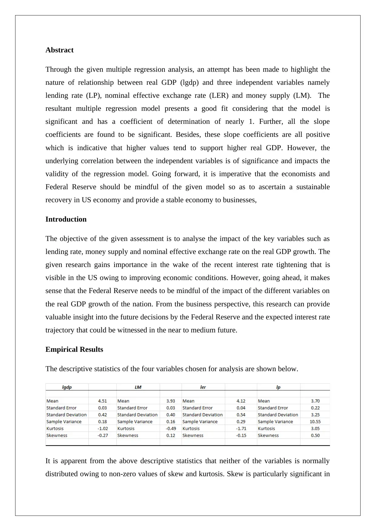
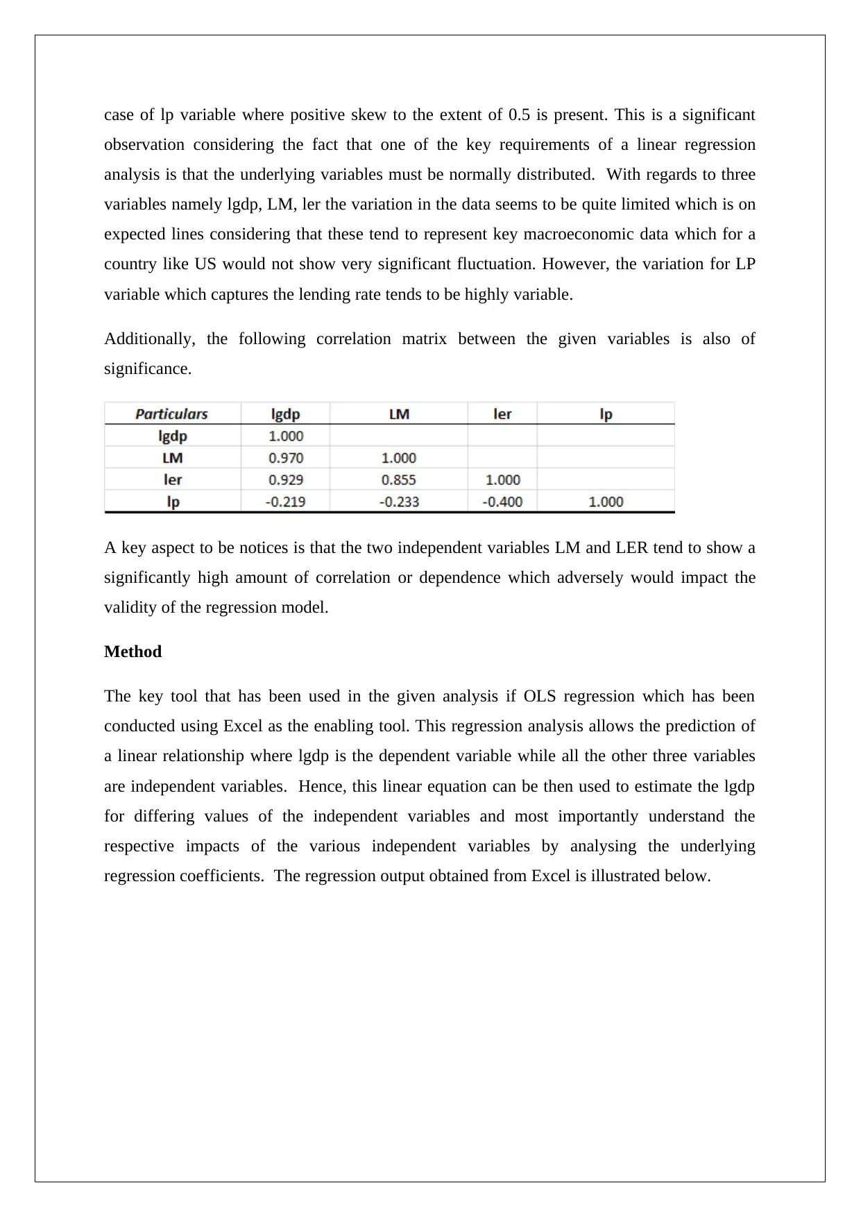
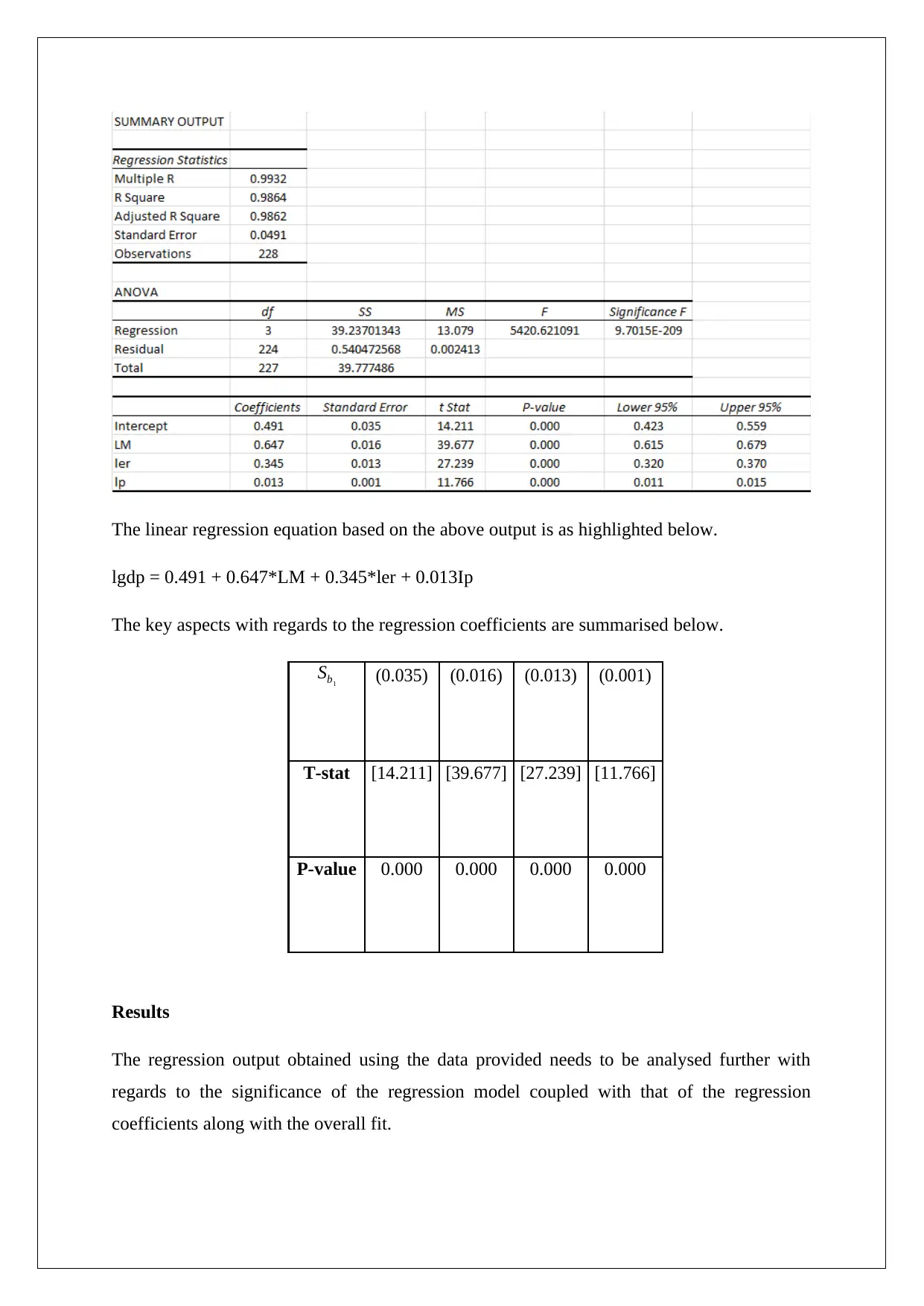
This project presents a multiple regression analysis to examine the relationship between US real GDP and three independent variables: lending rate, nominal effective exchange rate, and money supply. The analysis, conducted using Excel, reveals a significant and well-fitting model with a high coefficient of determination, indicating that nearly all variation in real GDP can be explained by the independent variables. All slope coefficients are statistically significant and positive, suggesting that higher values of these variables correlate with increased real GDP. However, the study acknowledges the high correlation between money supply and nominal effective exchange rate, which may impact the model's validity. The findings underscore the importance of considering these factors for sustainable economic recovery and stability, particularly for the Federal Reserve's decision-making. The project includes descriptive statistics, correlation analysis, and hypothesis testing to validate the model's significance and the significance of individual regression coefficients. The results suggest that the lending rate, money supply, and exchange rate are crucial determinants of real GDP, with implications for monetary policy and business decisions. This project is available on Desklib, a platform providing students with AI-based study tools, including past papers and solved assignments.

STATISTICS
STUDENT ID:
[Pick the date]

Abstract
Through the given multiple regression analysis, an attempt has been made to highlight the
nature of relationship between real GDP (lgdp) and three independent variables namely
lending rate (LP), nominal effective exchange rate (LER) and money supply (LM). The
resultant multiple regression model presents a good fit considering that the model is
significant and has a coefficient of determination of nearly 1. Further, all the slope
coefficients are found to be significant. Besides, these slope coefficients are all positive
which is indicative that higher values tend to support higher real GDP. However, the
underlying correlation between the independent variables is of significance and impacts the
validity of the regression model. Going forward, it is imperative that the economists and
Federal Reserve should be mindful of the given model so as to ascertain a sustainable
recovery in US economy and provide a stable economy to businesses,
Introduction
The objective of the given assessment is to analyse the impact of the key variables such as
lending rate, money supply and nominal effective exchange rate on the real GDP growth. The
given research gains importance in the wake of the recent interest rate tightening that is
visible in the US owing to improving economic conditions. However, going ahead, it makes
sense that the Federal Reserve needs to be mindful of the impact of the different variables on
the real GDP growth of the nation. From the business perspective, this research can provide
valuable insight into the future decisions by the Federal Reserve and the expected interest rate
trajectory that could be witnessed in the near to medium future.
Empirical Results
The descriptive statistics of the four variables chosen for analysis are shown below.
It is apparent from the above descriptive statistics that neither of the variables is normally
distributed owing to non-zero values of skew and kurtosis. Skew is particularly significant in

case of lp variable where positive skew to the extent of 0.5 is present. This is a significant
observation considering the fact that one of the key requirements of a linear regression
analysis is that the underlying variables must be normally distributed. With regards to three
variables namely lgdp, LM, ler the variation in the data seems to be quite limited which is on
expected lines considering that these tend to represent key macroeconomic data which for a
country like US would not show very significant fluctuation. However, the variation for LP
variable which captures the lending rate tends to be highly variable.
Additionally, the following correlation matrix between the given variables is also of
significance.
A key aspect to be notices is that the two independent variables LM and LER tend to show a
significantly high amount of correlation or dependence which adversely would impact the
validity of the regression model.
Method
The key tool that has been used in the given analysis if OLS regression which has been
conducted using Excel as the enabling tool. This regression analysis allows the prediction of
a linear relationship where lgdp is the dependent variable while all the other three variables
are independent variables. Hence, this linear equation can be then used to estimate the lgdp
for differing values of the independent variables and most importantly understand the
respective impacts of the various independent variables by analysing the underlying
regression coefficients. The regression output obtained from Excel is illustrated below.

The linear regression equation based on the above output is as highlighted below.
lgdp = 0.491 + 0.647*LM + 0.345*ler + 0.013Ip
The key aspects with regards to the regression coefficients are summarised below.
Sb1 (0.035) (0.016) (0.013) (0.001)
T-stat [14.211] [39.677] [27.239] [11.766]
P-value 0.000 0.000 0.000 0.000
Results
The regression output obtained using the data provided needs to be analysed further with
regards to the significance of the regression model coupled with that of the regression
coefficients along with the overall fit.

From the regression output, it is apparent the coefficient of determination or R2 has come out
as 0.9864. This indicates that 98.64% of the variation in the real GDP (dependent variable)
can be explained by corresponding variation in the given independent variables jointly. This
clearly shows an excellent fit considering the fact that the given multiple regression model is
not able to explain only 1.36% of the overall variation in the dependent variable (i.e. Real
GDP).
Additionally, hypothesis testing needs to be carried out in order to ascertain the significance
of the multiple regression model and the significance of the various regression coefficients.
This is carried out below.
Testing significance of the multiple regression model
The relevant hypotheses are as highlighted below.
Null Hypothesis: β1= β2= β3 =0 and hence the multiple regression model is insignificant.
Alternative Hypothesis: Atleast one of the slope coefficients in the given regression model is
not zero.
The relevant test statistic would be F test and a p value approach would be used. The
significance level has been assumed to be 5% 0r 0.05. The appropriate excel output to
highlight the F statistic and the corresponding p value is indicated below.
From the output shown above, it is evident that the F statistic is 5420.62 with a corresponding
p value of 0.00. Since the p value is lower than the applicable level of significance, hence it
would be appropriate to reject the null hypothesis and accept the alternative hypothesis.
Hence, this implies that there is atleast one independent variable which has a significant slope
owing to which the regression model is significant.
Testing significance of the Slope Coefficients
1) The relevant hypotheses are as highlighted below.

Null Hypothesis: βLM=0 i.e. the slope of LM variable can be assumed to be zero and hence
insignificant.
Alternative Hypothesis: βLM≠0 i.e. the slope of LM variable can be assumed to be zero and
hence insignificant.
The level of significance is taken as 5% or 0.05 for this test. Further, the relevant test
statistics would be t and the p value approach would be used. The t statistics and the p value
have been computed using regression model and amount to 39.677 and 0.000 respectively.
Since the p value is lower than the applicable level of significance, hence it would be
appropriate to reject the null hypothesis and accept the alternative hypothesis. Thus, it can be
concluded that the given slope coefficient is statistically significant and cannot be assumed as
zero.
2) The relevant hypotheses are as highlighted below.
Null Hypothesis: βler=0 i.e. the slope of ler variable can be assumed to be zero and hence
insignificant.
Alternative Hypothesis: βler≠0 i.e. the slope of ler variable can be assumed to be zero and
hence insignificant.
The level of significance is taken as 5% or 0.05 for this test. Further, the relevant test
statistics would be t and the p value approach would be used. The t statistics and the p value
have been computed using regression model and amount to 27.239 and 0.000 respectively.
Since the p value is lower than the applicable level of significance, hence it would be
appropriate to reject the null hypothesis and accept the alternative hypothesis. Thus, it can be
concluded that the given slope coefficient is statistically significant and cannot be assumed as
zero.
3) The relevant hypotheses are as highlighted below.
Null Hypothesis: βlp=0 i.e. the slope of lp variable can be assumed to be zero and hence
insignificant.
Alternative Hypothesis: βlp≠0 i.e. the slope of lp variable can be assumed to be zero and
hence insignificant.

The level of significance is taken as 5% or 0.05 for this test. Further, the relevant test
statistics would be t and the p value approach would be used. The t statistics and the p value
have been computed using regression model and amount to 11.766 and 0.000 respectively.
Since the p value is lower than the applicable level of significance, hence it would be
appropriate to reject the null hypothesis and accept the alternative hypothesis. Thus, it can be
concluded that the given slope coefficient is statistically significant and cannot be assumed as
zero.
Discussion
On the basis of the above results, it is apparent that with regards to determination of real
GDP, all the given three variables are significant and tend to almost offer explanation for
100% of the variation in GDP. Considering that the coefficients of all the three independent
variables are positive, it would imply that increasing these would increase the real GDP. One
of these is the money supply and increasing this clearly would lead to higher real GDP as was
the case during quantitative easing when the focus was on ensuring enough liquidity in the
system. Apparently higher liquidity in the system would automatically lead to lowering of the
lending rates which reflects a sought of balance between the independent variables which
cannot be all increased at the same time owing to economic constraints. Also, on account of
high correlation of 0.855 between money supply and nominal effective exchange rate, these
two variables essentially can be captured through the money supply only. Hence, going
forward as the interest rate hardening continues by the Federal Reserve, it ought to be
mindful of the fact that adverse impact on availability of liquidity could lead to adverse
impact on real GDP and hence needs to prudent and balance in its approach.