Macquarie University STAT821/STAT721 Multivariate Analysis Exam 2017

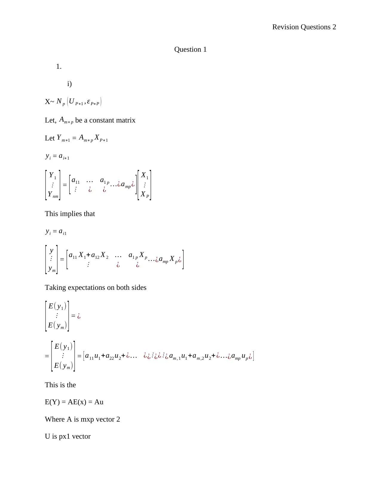
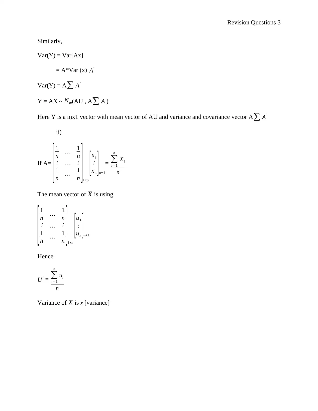
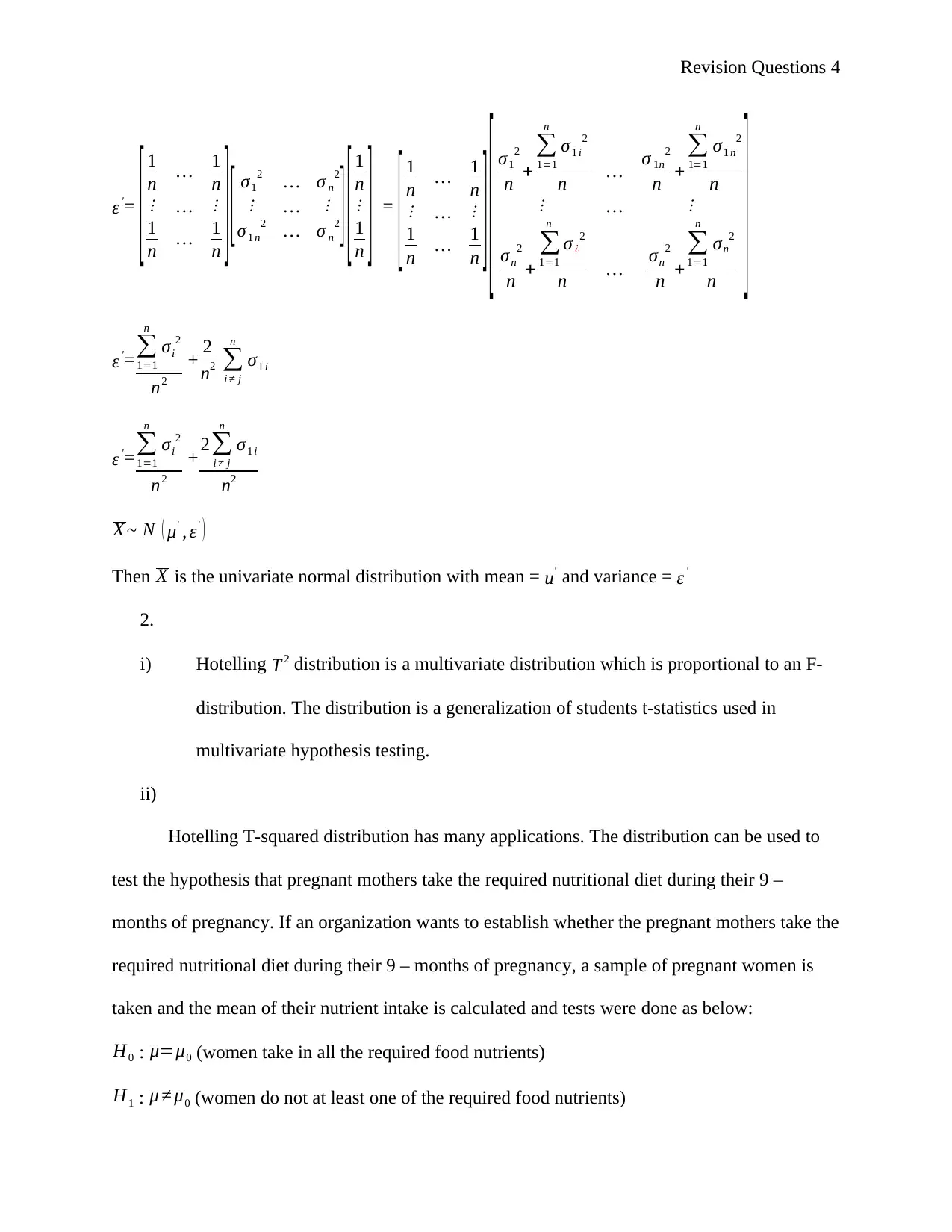
This document provides solutions to revision questions for a Multivariate Analysis exam (STAT821/STAT721). The questions cover topics such as the distribution of linear transformations of normally distributed variables, the application and assumptions of Hotelling's T-squared distribution with a nutritional diet case study, the usefulness and construction of Q-Q plots for assessing normality, simultaneous confidence intervals, hypothesis testing with dependent random variables using t-tests, principal component analysis, and least squares estimation in multiple regression models including hypothesis testing and confidence interval construction. The solutions demonstrate the application of statistical concepts and techniques to solve problems in multivariate analysis.

Revision Questions 1
Exam Revision November 2017
(Student Name)
Course
Professor
Institution
City and State of the University
Date

Revision Questions 2
Question 1
1.
i)
X~ N p ( U P∗1 , ε P∗P )
Let, Am∗ p be a constant matrix
Let Y m∗1 = Am∗ p XP∗1
yi = ai∗1
[ Y 1
⋮
Y nm ] = [a11 … a1 p
⋮ ¿ ¿ …¿amp ¿ ] [ X1
⋮
X P ]
This implies that
yi = ai1
[ y
⋮
ym ] = [a11 X1+ a12 X 2 … a1 p X p
⋮ ¿ ¿ …¿amp X p ¿ ]
Taking expectations on both sides
[ E( y1 )
⋮
E( ym ) ] = ¿
= [ E( y1 )
⋮
E( ym ) ] = [ a11 u1 +a22 u2+¿ … ¿¿ ⋮ ¿¿ ⋮ ¿ am , 1 u1 +am ,2 u2+¿ …¿amp up ¿ ]
This is the
E(Y) = AE(x) = Au
Where A is mxp vector 2
U is px1 vector

Revision Questions 3
Similarly,
Var(Y) = Var[Ax]
= A*Var (x) A'
Var(Y) = A∑ A'
Y = AX ~ Nm(AU , A∑ A')
Here Y is a mx1 vector with mean vector of AU and variance and covariance vector A ∑ A'
ii)
If A=
[ 1
n … 1
n
⋮ … ⋮
1
n … 1
n ]1 xp
[ x1
⋮
xn ] n∗1
= ∑
i=1
n
Xi
n
The mean vector of X is using
[ 1
n … 1
n
⋮ … ⋮
1
n … 1
n ]1 xn
[ u1
⋮
un ]u∗1
Hence
U' = ∑
i=1
n
ui
n
Variance of X is ε '[variance]

Revision Questions 4
ε '=
[ 1
n … 1
n
⋮ … ⋮
1
n … 1
n ] [ σ1
2 … σ n
2
⋮ … ⋮
σ1 n
2 … σ n
2 ] [ 1
n
⋮
1
n ] =
[ 1
n … 1
n
⋮ … ⋮
1
n … 1
n ] [ σ1
2
n +
∑
1=1
n
σ1 i
2
n … σ 1n
2
n +
∑
1=1
n
σ1 n
2
n
⋮ … ⋮
σn
2
n +
∑
1=1
n
σ ¿
2
n … σn
2
n +
∑
1=1
n
σn
2
n
]
ε '=∑
1=1
n
σi
2
n2
+ 2
n2 ∑
i ≠ j
n
σ1 i
ε '= ∑
1=1
n
σi
2
n2
+ 2∑
i ≠ j
n
σ1 i
n2
X ~ N ( μ' , ε' )
Then X is the univariate normal distribution with mean = u' and variance = ε '
2.
i) Hotelling T 2 distribution is a multivariate distribution which is proportional to an F-
distribution. The distribution is a generalization of students t-statistics used in
multivariate hypothesis testing.
ii)
Hotelling T-squared distribution has many applications. The distribution can be used to
test the hypothesis that pregnant mothers take the required nutritional diet during their 9 –
months of pregnancy. If an organization wants to establish whether the pregnant mothers take the
required nutritional diet during their 9 – months of pregnancy, a sample of pregnant women is
taken and the mean of their nutrient intake is calculated and tests were done as below:
H0 : μ=μ0 (women take in all the required food nutrients)
H1 : μ ≠ μ0 (women do not at least one of the required food nutrients)

Revision Questions 5
Assumptions made for the univariate case
a) Only one single nutritional component is measured
b) Homoskedasticity (Equality of variance) is assumed
c) The variables are independent (Independence assumption )
d) Normality of subjects is assumed
Since this is a univariate test, the test statistics are calculated as below:
t=
x−μ0
√ s2
n
~ tn−1
The null hypothesis follows the t-distribution.
Decision rule: Reject the null hypothesis id the observed/calculated t value is greater than the t
critical value
|t|> tn−1 , α
2
Summary
In question 2 part(ii) , I have given a case study or example where Hotelling t squared
distribution is practically applied then I have constructed possible hypothesis from the case
study . I also stated all the assumptions of Hotelling t squared , test statistic and he distribution it
follows.
3.
Usefulness of a Q-Q plot
i. Graphic representation of Q-Q plot assists in testing for normality
ii. The presence or absence of outliers in Q-Q plot assists in knowing the how
symmetrical a data sequence is to the normal distribution
Construction of Q-Q plot

Revision Questions 6
i. Arrange values in an ascending order
ii. Draw a normal distribution curve into n+1 segments
iii. Find the z-value for every segment
4.
Simultaneous (1- α)*100% T 2 the confidence interval is used to calculate a confidence interval
for linear combinations of linear variables.
y j ± √ p(n−1)
n− p F p ,n− p , α
√ SY
2
n
Bonferroni (1- α )*100% confidence interval is used to calculate confidence interval s or
individual variables.
y j
± tn −1 , α
2 p √ SY
2
n
Number 2
1.
Random variables T 1, T 2, T 3, T 4 are dependent given ,
X= ( T 1
⋮
T n
) ~ N
( μ1
⋮
μn
, ϵ
) y = ( μ1
⋮
μn
)
H0: μ = μ1+μ2+ μ3
3 ⟹ 3 μ1- μ2- μ3-μ4
Thus
A = (3,-1,-1,-1)
i)
When n is small, we cannot use the normality test , so
Let X1 → X2 be a 4-dimensional sample

Revision Questions 7
Let Y 1= AX1, i= I 1(n)
E( Y i) = A.E( Xi) = A. μ = 0
We can estimate, ^σ y
2 = 1
n−1 ∑
i=1
m
( yi− y)2
= 1
n−1 ∑
i=1
m
( A Xi −A X )2
= 1
n−1 ∑
i=1
m
( A Xi −A X )(A Xi− A X )'
= 1
n−1 ∑
i=1
m
A (Xi −X )(Xi− X )' A'
= A [ ∑
i=1
m
A ( Xi−X )(Xi −X )'
] A'
According to standard t-test ;
T =
Y
( ^σ y
√ n ) ~ tn−1
(T=
Y
( ^σ y
√n ) = √n A X
^σ y
)
The technique is to transform Xis to univariates by the use standard t-test
ii)
When n is large, the same technique as in part (i) above is used but with an additional result.
For large n, S= 1
n−1 ∑
i=1
m
( X i−X )( Xi −X )' ⟶ ε almost surely
Through continuous mapping theorem,
^σ y= √ AS A' ⟶ √ A ∑ A' almost surely

Revision Questions 8
Using continuous mapping theorem which states that if x⟶a with probability p and g() is a
function with finite discontinuities then g' ¿) x⟶ g(a) almost surely
A X ~ N(0, A ∑ A'
n )= √ n A X
√ A ∑ A' ~ N(0,1) and √ A ∑ A'
√ AS A' ⟶ 1 almost surely
So, ( √n A Y
√ A ∑ A' ) ( √ A ∑ A'
√ AS A' ) = √n A X
√ AS A' ~ N(0,1)
2.
We use t-distribution in this question
Since this is a univariate test, the test statistics is calculated as below:
t=
x−μ0
√ s2
n
~ tn−1
The null hypothesis follows the t-distribution.
Decision rule: Reject the null hypothesis id the observed/calculated t value is greater than the t
critical value
|t|> tn−1 , α
2
Number 3
1.
Y 1 = e1
' X = -0.383X1 +-0.924 X2
Y 2 = e1
' X = -0.924 X1 +-0.383 X2
2.
Principal component Y 1
λ1
λ1 + λ2
= 5.828
5.828+0.172 = 0.9713

Revision Questions 9
Principal component Y 3
λ2
λ1 + λ2
= 0.172
5.828+0.172 = 0.0287
3.
No correlation between X and Y 2 . The principal component Y 2 explains 2.87% of the total
population variance.
Question 4
1.
The equation can be written down in a matrix form as;
Y = X β + ε
Where
Y = ( y1 , y2 … . yn)'
X= X = [1 X21 X31
⋮ ⋮ ⋮
1 X2 n X3 n ] β = [ β0
⋮
β2 ] ε = [ε0
⋮
ε2 ]
Thus the least estimators of β are
^β = (X' X )−1 X'Y , ^Y = X ^β
^εreduced = (y- ^y) ⟹ ∑ εi
2 = ( y− ^y)1(y- ^y)
The degrees of freedom for error sum of squares are -3
Test statistic
F =
(error ∑ of squares for reduced model−error ∑ of squares for full model)
( Error ∑ of squares for full model
n−4 )

Revision Questions 10
F=
( y − ^y)1 ( y − ^y)
( X β +ε
n−4 )
2.
Suppose β2=β3= 0
Then,
y1 = β0 + β2 X1 i + ε i
X = ¿
Then
^β = (X' X )−1 X'Y
^Y = X ^β
^εreduced = (y- ^y) ⟹ ∑ εi
2 = ( y− ^y)1(y- ^y) …..
The test statistic, F is calculated as
F=
(∑ εi
2 reduced−∑ ε i
2 full)
2
((∑ εi
2 full)
n−4 )
3.
The confidence interval for β2−β3 is calculated as:
{√ ^σ2
√ a' (X ' X )−1 a}tn−4 ± a' ^β
Here
a=[0 0 1−1]'
x is a matrix design under full model
^σ 2 is ∑ εi
2 full
n−4

Revision Questions 11
^β is estimated in full model
tn−4 is critical value of t distribution . At 95% confidence interval, tn−4 is calculated as;
P(t> tn−4) = 0.025