Predictive Analytics Project: NBA Win and Playoff Predictions
VerifiedAdded on 2021/12/20
|14
|1531
|49
Project
AI Summary
This project utilizes predictive analytics to forecast the performance of NBA teams, specifically focusing on predicting wins and playoff appearances for the 2016-2017 and 2017-2018 seasons. The project employs multiple regression and classification modeling techniques using historical NBA data. Initially, the win/loss proxy stats were dropped. The multiple regression model was developed to predict wins based on variables such as age, offensive rating, defensive rating, turnover %, true shooting %, effective field goal %, and offensive rebound %. Through iterative refinement, the most effective model (Model 3) was identified, accounting for 95.13% of the variability and including age, offensive rating, defensive rating, and opponent effective field goal. The margin of error was calculated. Furthermore, classification modeling, particularly decision trees, was used to determine which teams would qualify for the playoffs, with the data split into training and test datasets. The decision tree model provided rules for playoff qualification based on net rating. The project compares the predicted and actual values of the models and applies the models to the 2018-2019 data. References to relevant literature are also provided.
Introduction
Predictive analytics is often viewed as a segment of data analytics whose role is majorly
to determine a set of unknown future values given historical data. In an article on the role of
predictive analytics, Batterham, Christensen, and Mackinnon (2009) note that, “…the science of
predictive analytics can generate future insights with a significant degree of precision.”
Therefore, well defined and logical models are crucial in offering significant forecast on future
performance on virtually any endeavor as long as there is reliable data.
Elsewhere, Hastie, Tibshirani and Friedman (2001) define predictive analytics as a
stepwise method of examining meaningful information from data using specified tools and
methodologies.
However, in the world of data, it is not always true that complete historical data will
always available. In such scenarios, predictive analytics is essentially the best option to enable
precise re-imaging of how the original outcome would be given ideal conditions.
Purpose of project
The purpose of this paper is therefore to employ the use of logical and well defined
predictive analytics tools to predict the performance of the teams in the 2016-2017 and 2017-
2018 seasons of the NBA using historical data given the loss of win and loss data. As such, the
project outcomes will include prediction of wins and determining which teams will be in the
playoffs in the 2016-2017 and 2017-2018 seasons.
Paraphrase This Document
Need a fresh take? Get an instant paraphrase of this document with our AI Paraphraser
Predictive modeling
Given the above argument, it is clear that in predictive modeling, the main objective is to
predict the outcome of a single response variable, say Y, given either multiple or a single
predictor variable X.
Multiple regression predictive tool
One of the methods used in analysis of relationships between different factors is linear
regression. In simple linear regression, a single response variable is assumed to be linearly
related to a single predictor variable. In contrast, multiple linear regression is used to examine
the relationship between a single response variable with multiple predictor variables hence the
model of the form:
Yi = α + β1Xi,1 + · · · + βpXi,p + £i Where ; α= Y intercept, βi, i=1,2,…, p are the
regressors coefficients and Xi are the predictor
variables.
Given the purpose of the project, multiple linear regression will be the effective tool for
predicting future wins given historical data.
Process of multiple regression modeling
Initially, the win/loss proxy stats from the historical data are dropped due to their effect
on the prediction outcome. Now, in prediction of the NBA wins for the seasons 2010-2011 to
2015-2016, the following multiple regression model is adopted:
Win= α + β1Age+ β2 Offensive Rating+ β3 Defensive Rating+ β4 Offensive Rebound+...+ β16
Turnover %
SUMMARY OUTPUT
Regression Statistics
Multiple R 0.95382
R Square 0.909773
Adjusted R0.900917
Standard E4.079699
Observatio 180
ANOVA
df SS MS F Significance F
Regression 16 27355.37 1709.71 102.7227 2.49E-76
Residual 163 2712.963 16.64394
Total 179 30068.33
CoefficientsStandard Error t Stat P-value Lower 95%Upper 95%Lower 95.0%Upper 95.0%
Intercept -161.164 150.8347 -1.06848 0.286883 -459.006 136.6778 -459.006 136.6778
Age 0.681496 0.221691 3.074084 0.002476 0.24374 1.119252 0.24374 1.119252
Offensive R2.113902 1.811313 1.167055 0.244893 -1.46276 5.690565 -1.46276 5.690565
Defensive -0.80814 1.509823 -0.53526 0.593203 -3.78947 2.173193 -3.78947 2.173193
Offensive 0.04298 0.967672 0.044416 0.964627 -1.86781 1.953768 -1.86781 1.953768
Free throw -47.8179 50.44918 -0.94784 0.344613 -147.436 51.8003 -147.436 51.8003
1.697983 2.039191 0.832675 0.406247 -2.32865 5.724619 -2.32865 5.724619
Opp Effecti -173.196 236.1274 -0.73349 0.464316 -639.459 293.067 -639.459 293.067
Free Throw-78.9851 284.5738 -0.27756 0.781705 -640.911 482.9412 -640.911 482.9412
3-Point At 3.994306 12.45832 0.320614 0.748914 -20.6062 28.59481 -20.6062 28.59481
Free Throw33.38872 138.7253 0.240682 0.810104 -240.542 307.3192 -240.542 307.3192
Effective F -171.814 562.0798 -0.30568 0.760241 -1281.71 938.0821 -1281.71 938.0821
Defensive 0.930437 0.785285 1.18484 0.237805 -0.62021 2.48108 -0.62021 2.48108
Net Rating 0.015544 0.009414 1.651138 0.100636 -0.00305 0.034132 -0.00305 0.034132
247.3421 684.8978 0.361137 0.718464 -1105.07 1599.758 -1105.07 1599.758
Pace Facto 0.119268 0.151237 0.788617 0.431481 -0.17937 0.417905 -0.17937 0.417905
Opponent Turnover
True Shooting%
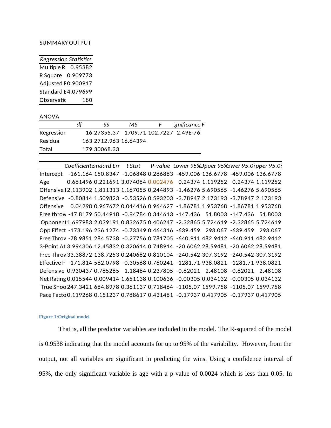
Figure 1:Original model
That is, all the predictor variables are included in the model. The R-squared of the model
is 0.9538 indicating that the model accounts for up to 95% of the variability. However, from the
output, not all variables are significant in predicting the wins. Using a confidence interval of
95%, the only significant variable is age with a p-value of 0.0024 which is less than 0.05. In
Regression Statistics
Multiple R 0.95382
R Square 0.909773
Adjusted R0.900917
Standard E4.079699
Observatio 180
ANOVA
df SS MS F Significance F
Regression 16 27355.37 1709.71 102.7227 2.49E-76
Residual 163 2712.963 16.64394
Total 179 30068.33
CoefficientsStandard Error t Stat P-value Lower 95%Upper 95%Lower 95.0%Upper 95.0%
Intercept -161.164 150.8347 -1.06848 0.286883 -459.006 136.6778 -459.006 136.6778
Age 0.681496 0.221691 3.074084 0.002476 0.24374 1.119252 0.24374 1.119252
Offensive R2.113902 1.811313 1.167055 0.244893 -1.46276 5.690565 -1.46276 5.690565
Defensive -0.80814 1.509823 -0.53526 0.593203 -3.78947 2.173193 -3.78947 2.173193
Offensive 0.04298 0.967672 0.044416 0.964627 -1.86781 1.953768 -1.86781 1.953768
Free throw -47.8179 50.44918 -0.94784 0.344613 -147.436 51.8003 -147.436 51.8003
1.697983 2.039191 0.832675 0.406247 -2.32865 5.724619 -2.32865 5.724619
Opp Effecti -173.196 236.1274 -0.73349 0.464316 -639.459 293.067 -639.459 293.067
Free Throw-78.9851 284.5738 -0.27756 0.781705 -640.911 482.9412 -640.911 482.9412
3-Point At 3.994306 12.45832 0.320614 0.748914 -20.6062 28.59481 -20.6062 28.59481
Free Throw33.38872 138.7253 0.240682 0.810104 -240.542 307.3192 -240.542 307.3192
Effective F -171.814 562.0798 -0.30568 0.760241 -1281.71 938.0821 -1281.71 938.0821
Defensive 0.930437 0.785285 1.18484 0.237805 -0.62021 2.48108 -0.62021 2.48108
Net Rating 0.015544 0.009414 1.651138 0.100636 -0.00305 0.034132 -0.00305 0.034132
247.3421 684.8978 0.361137 0.718464 -1105.07 1599.758 -1105.07 1599.758
Pace Facto 0.119268 0.151237 0.788617 0.431481 -0.17937 0.417905 -0.17937 0.417905
Opponent Turnover
True Shooting%
Figure 1:Original model
That is, all the predictor variables are included in the model. The R-squared of the model
is 0.9538 indicating that the model accounts for up to 95% of the variability. However, from the
output, not all variables are significant in predicting the wins. Using a confidence interval of
95%, the only significant variable is age with a p-value of 0.0024 which is less than 0.05. In
⊘ This is a preview!⊘
Do you want full access?
Subscribe today to unlock all pages.
Trusted by 1+ million students worldwide
order to determine the significance of each variable, every predictor variable is examined
individually.
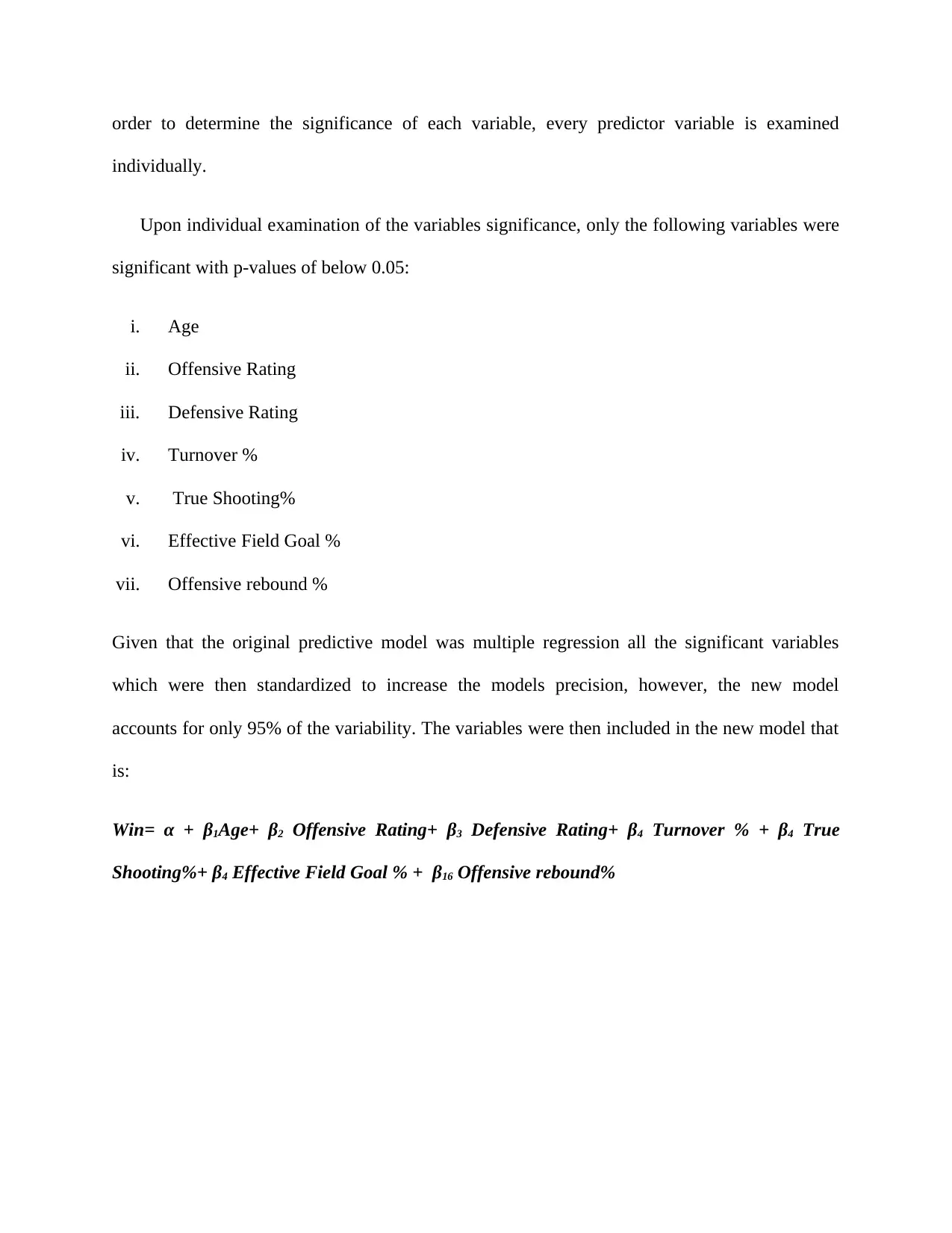
Upon individual examination of the variables significance, only the following variables were
significant with p-values of below 0.05:
i. Age
ii. Offensive Rating
iii. Defensive Rating
iv. Turnover %
v. True Shooting%
vi. Effective Field Goal %
vii. Offensive rebound %
Given that the original predictive model was multiple regression all the significant variables
which were then standardized to increase the models precision, however, the new model
accounts for only 95% of the variability. The variables were then included in the new model that
is:
Win= α + β1Age+ β2 Offensive Rating+ β3 Defensive Rating+ β4 Turnover % + β4 True
Shooting%+ β4 Effective Field Goal % + β16 Offensive rebound%
individually.
Upon individual examination of the variables significance, only the following variables were
significant with p-values of below 0.05:
i. Age
ii. Offensive Rating
iii. Defensive Rating
iv. Turnover %
v. True Shooting%
vi. Effective Field Goal %
vii. Offensive rebound %
Given that the original predictive model was multiple regression all the significant variables
which were then standardized to increase the models precision, however, the new model
accounts for only 95% of the variability. The variables were then included in the new model that
is:
Win= α + β1Age+ β2 Offensive Rating+ β3 Defensive Rating+ β4 Turnover % + β4 True
Shooting%+ β4 Effective Field Goal % + β16 Offensive rebound%
Paraphrase This Document
Need a fresh take? Get an instant paraphrase of this document with our AI Paraphraser
SUMMARY OUTPUT
Regression Statistics
Multiple R 0.951526
R Square 0.905401
Adjusted R0.901551
Standard E4.066618
Observatio 180
ANOVA
df SS MS F Significance F
Regression 7 27223.9 3889.128 235.171974 1.43E-84
Residual 172 2844.429 16.53738
Total 179 30068.33
CoefficientsStandard Error t Stat P-value Lower 95%Upper 95%Lower 95.0%Upper 95.0%
Intercept -11.4412 24.60521 -0.46499 0.642527097 -60.0082 37.12589 -60.0082 37.12589
Age 0.552282 0.199986 2.761598 0.00637685 0.157538 0.947025 0.157538 0.947025
Offensive R1.674706 1.084614 1.544058 0.024412227 -0.46616 3.815574 -0.46616 3.815574
Defensive -2.00284 0.110877 -18.0637 1.39874E-41 -2.2217 -1.78399 -2.2217 -1.78399
Offensive 0.18273 0.567398 0.32205 0.74780625 -0.93723 1.30269 -0.93723 1.30269
Turnover -1.27463 1.526079 -0.83523 0.404747699 -4.28688 1.73763 -4.28688 1.73763
158.9237 191.3505 0.830537 0.407386634 -218.774 536.6213 -218.774 536.6213
Effective F -3.21005 57.94648 -0.0554 0.95588666 -117.588 111.1677 -117.588 111.1677
True Shooting%
22 23 24
-15
-10
-5
0
5
10
15
Age
Residuals
Figure 2: Model 2
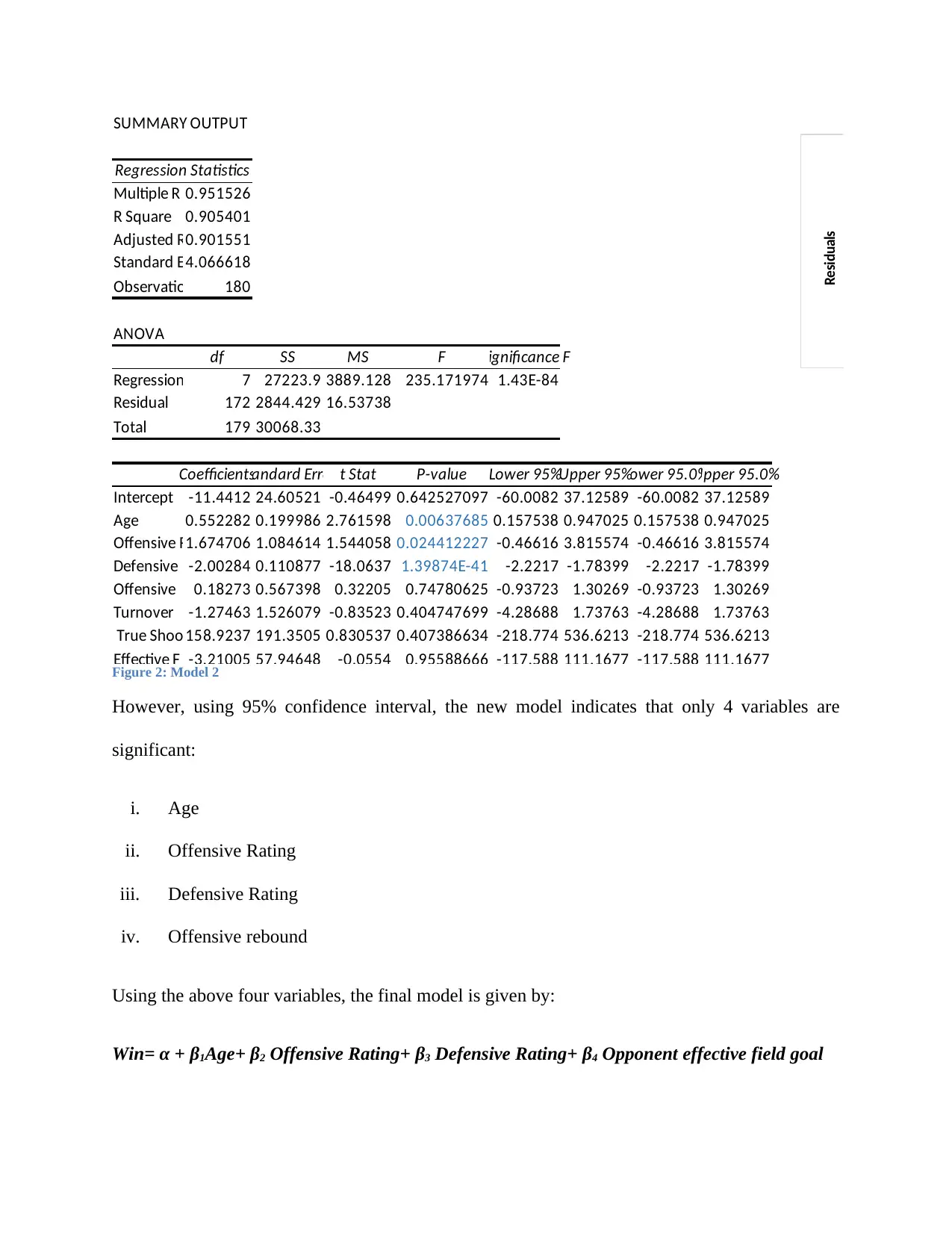
However, using 95% confidence interval, the new model indicates that only 4 variables are
significant:
i. Age
ii. Offensive Rating
iii. Defensive Rating
iv. Offensive rebound
Using the above four variables, the final model is given by:
Win= α + β1Age+ β2 Offensive Rating+ β3 Defensive Rating+ β4 Opponent effective field goal
Regression Statistics
Multiple R 0.951526
R Square 0.905401
Adjusted R0.901551
Standard E4.066618
Observatio 180
ANOVA
df SS MS F Significance F
Regression 7 27223.9 3889.128 235.171974 1.43E-84
Residual 172 2844.429 16.53738
Total 179 30068.33
CoefficientsStandard Error t Stat P-value Lower 95%Upper 95%Lower 95.0%Upper 95.0%
Intercept -11.4412 24.60521 -0.46499 0.642527097 -60.0082 37.12589 -60.0082 37.12589
Age 0.552282 0.199986 2.761598 0.00637685 0.157538 0.947025 0.157538 0.947025
Offensive R1.674706 1.084614 1.544058 0.024412227 -0.46616 3.815574 -0.46616 3.815574
Defensive -2.00284 0.110877 -18.0637 1.39874E-41 -2.2217 -1.78399 -2.2217 -1.78399
Offensive 0.18273 0.567398 0.32205 0.74780625 -0.93723 1.30269 -0.93723 1.30269
Turnover -1.27463 1.526079 -0.83523 0.404747699 -4.28688 1.73763 -4.28688 1.73763
158.9237 191.3505 0.830537 0.407386634 -218.774 536.6213 -218.774 536.6213
Effective F -3.21005 57.94648 -0.0554 0.95588666 -117.588 111.1677 -117.588 111.1677
True Shooting%
22 23 24
-15
-10
-5
0
5
10
15
Age
Residuals
Figure 2: Model 2
However, using 95% confidence interval, the new model indicates that only 4 variables are
significant:
i. Age
ii. Offensive Rating
iii. Defensive Rating
iv. Offensive rebound
Using the above four variables, the final model is given by:
Win= α + β1Age+ β2 Offensive Rating+ β3 Defensive Rating+ β4 Opponent effective field goal
SUMMARY OUTPUT
Regression Statistics
Multiple R 0.995365
R Square 0.990752
Adjusted R0.984912
Standard E4.056907
Observatio 180
ANOVA
df SS MS F Significance F
Regression 4 310312 77578.08 4713.559 5.7E-177
Residual 176 2896.695 16.45849
Total 180 313209
CoefficientsStandard Error t Stat P-value Lower 95%Upper 95%Lower 95.0%Upper 95.0%
Intercept 0 #N/A #N/A #N/A #N/A #N/A #N/A #N/A
Age 0.442925 0.184701 2.398073 0.017527 0.078412 0.807438 0.078412 0.807438
Offensive R 2.49642 0.085205 29.29885 1.35E-69 2.328264 2.664575 2.328264 2.664575
Defensive -2.15813 0.062015 -34.8002 8.1E-81 -2.28052 -2.03574 -2.28052 -2.03574
Figure 3: Model 3
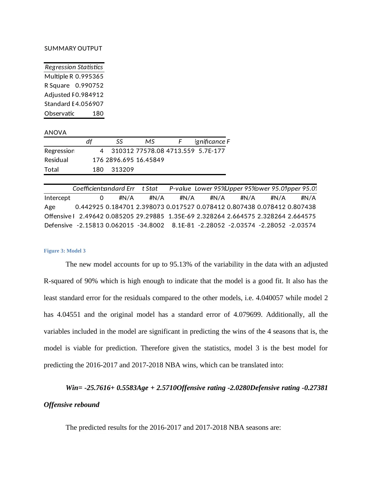
The new model accounts for up to 95.13% of the variability in the data with an adjusted
R-squared of 90% which is high enough to indicate that the model is a good fit. It also has the
least standard error for the residuals compared to the other models, i.e. 4.040057 while model 2
has 4.04551 and the original model has a standard error of 4.079699. Additionally, all the
variables included in the model are significant in predicting the wins of the 4 seasons that is, the
model is viable for prediction. Therefore given the statistics, model 3 is the best model for
predicting the 2016-2017 and 2017-2018 NBA wins, which can be translated into:
Win= -25.7616+ 0.5583Age + 2.5710Offensive rating -2.0280Defensive rating -0.27381
Offensive rebound
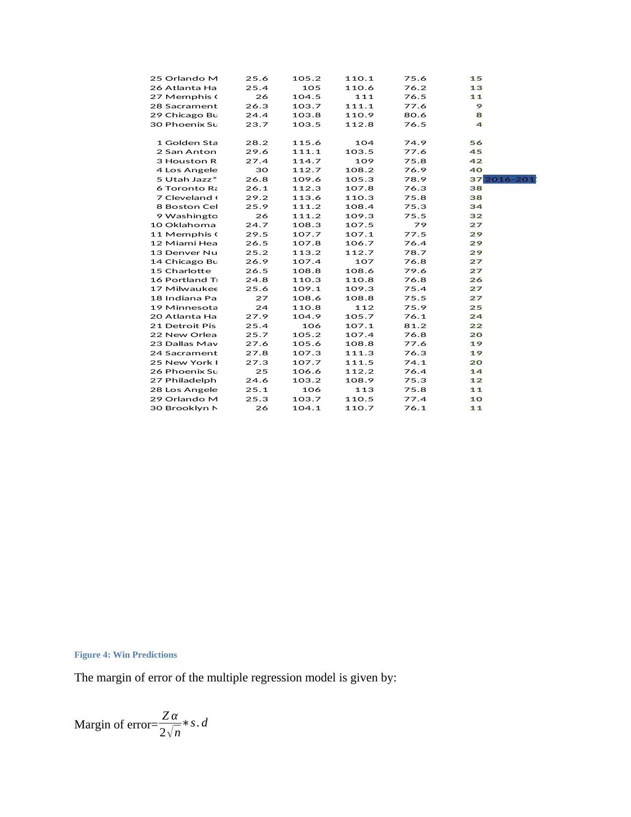
The predicted results for the 2016-2017 and 2017-2018 NBA seasons are:
Regression Statistics
Multiple R 0.995365
R Square 0.990752
Adjusted R0.984912
Standard E4.056907
Observatio 180
ANOVA
df SS MS F Significance F
Regression 4 310312 77578.08 4713.559 5.7E-177
Residual 176 2896.695 16.45849
Total 180 313209
CoefficientsStandard Error t Stat P-value Lower 95%Upper 95%Lower 95.0%Upper 95.0%
Intercept 0 #N/A #N/A #N/A #N/A #N/A #N/A #N/A
Age 0.442925 0.184701 2.398073 0.017527 0.078412 0.807438 0.078412 0.807438
Offensive R 2.49642 0.085205 29.29885 1.35E-69 2.328264 2.664575 2.328264 2.664575
Defensive -2.15813 0.062015 -34.8002 8.1E-81 -2.28052 -2.03574 -2.28052 -2.03574
Figure 3: Model 3
The new model accounts for up to 95.13% of the variability in the data with an adjusted
R-squared of 90% which is high enough to indicate that the model is a good fit. It also has the
least standard error for the residuals compared to the other models, i.e. 4.040057 while model 2
has 4.04551 and the original model has a standard error of 4.079699. Additionally, all the
variables included in the model are significant in predicting the wins of the 4 seasons that is, the
model is viable for prediction. Therefore given the statistics, model 3 is the best model for
predicting the 2016-2017 and 2017-2018 NBA wins, which can be translated into:
Win= -25.7616+ 0.5583Age + 2.5710Offensive rating -2.0280Defensive rating -0.27381
Offensive rebound
The predicted results for the 2016-2017 and 2017-2018 NBA seasons are:
⊘ This is a preview!⊘
Do you want full access?
Subscribe today to unlock all pages.
Trusted by 1+ million students worldwide
25 Orlando Ma 25.6 105.2 110.1 75.6 15
26 Atlanta Ha 25.4 105 110.6 76.2 13
27 Memphis Gr 26 104.5 111 76.5 11
28 Sacramento 26.3 103.7 111.1 77.6 9
29 Chicago Bul 24.4 103.8 110.9 80.6 8
30 Phoenix Su 23.7 103.5 112.8 76.5 4
1 Golden Sta 28.2 115.6 104 74.9 56
2 San Antoni 29.6 111.1 103.5 77.6 45
3 Houston Ro 27.4 114.7 109 75.8 42
4 Los Angeles 30 112.7 108.2 76.9 40
5 Utah Jazz* 26.8 109.6 105.3 78.9 37 2016-2017
6 Toronto Ra 26.1 112.3 107.8 76.3 38
7 Cleveland C 29.2 113.6 110.3 75.8 38
8 Boston Celt 25.9 111.2 108.4 75.3 34
9 Washingto 26 111.2 109.3 75.5 32
10 Oklahoma C 24.7 108.3 107.5 79 27
11 Memphis Gr 29.5 107.7 107.1 77.5 29
12 Miami Hea 26.5 107.8 106.7 76.4 29
13 Denver Nu 25.2 113.2 112.7 78.7 29
14 Chicago Bul 26.9 107.4 107 76.8 27
15 Charlotte 26.5 108.8 108.6 79.6 27
16 Portland Tr 24.8 110.3 110.8 76.8 26
17 Milwaukee 25.6 109.1 109.3 75.4 27
18 Indiana Pa 27 108.6 108.8 75.5 27
19 Minnesota 24 110.8 112 75.9 25
20 Atlanta Ha 27.9 104.9 105.7 76.1 24
21 Detroit Pis 25.4 106 107.1 81.2 22
22 New Orlean 25.7 105.2 107.4 76.8 20
23 Dallas Mav 27.6 105.6 108.8 77.6 19
24 Sacramento 27.8 107.3 111.3 76.3 19
25 New York K 27.3 107.7 111.5 74.1 20
26 Phoenix Su 25 106.6 112.2 76.4 14
27 Philadelphi 24.6 103.2 108.9 75.3 12
28 Los Angele 25.1 106 113 75.8 11
29 Orlando Ma 25.3 103.7 110.5 77.4 10
30 Brooklyn N 26 104.1 110.7 76.1 11
Figure 4: Win Predictions
The margin of error of the multiple regression model is given by:
Margin of error= Z α
2 √n∗s . d
Paraphrase This Document
Need a fresh take? Get an instant paraphrase of this document with our AI Paraphraser
Where n is the sample population, Zα is the Z-test statistical value at 95% confidence interval and
s.d . Therefore;
Margin of error= 1.96
√180 ∗4.040057
The margin of error for model three is 0.5902.
Classification modeling
Classification modeling is mainly concerned with class identification. Brownlee (2017) argues
that, the main difference between classification modeling and regression modeling that,
“fundamentally, classification is about predicting a label and regression is about predicting a
quantity.”
Therefore in classification modeling, the aim is to define rules with which to apply to subject
data in order to determine the teams that will be in the playoffs.
Decision tree
Decision tree models are often employed in connecting classification models given multiple
covariates as well as coming up with prediction methods for a given target variable, in this case,
which teams will be in the playoffs. The method, “…classifies a population into branch-like
segments that construct an inverted tree with a root node, internal nodes, and leaf nodes.” (Song
and LU, 2015).
Data training
The subject data is spitted into training and test datasets as in the figure below:
Classification Tree Model
Tree Information
Number of Training observations 50
Number of Test observations 10 Total Number of Nodes 2
Number of Leaf Nodes 2
Number of Predictors 17 Number of Levels 2
Class Variable Playoff % Missclasssified
Number of Classes 2 On Training Data 0.00%
Majority Class no On Test Data 0.00%
% MissClassified if Majority Class Time Taken
is used as Predicted Class 27% Data Processing 6 Sec
Tree Growing 23 Sec
Tree Pruning 0 Sec
Tree Drawing 1 Sec
Classification using final tree 3 Sec
Rule Generation 2 Sec
Confusion Matrix Total 36 Sec
Training Data Test Data
Predicted Class Predicted Class
True Class no yes True Class no yes
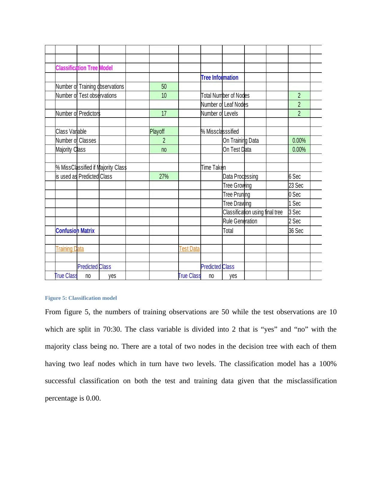
Figure 5: Classification model
From figure 5, the numbers of training observations are 50 while the test observations are 10
which are split in 70:30. The class variable is divided into 2 that is “yes” and “no” with the
majority class being no. There are a total of two nodes in the decision tree with each of them
having two leaf nodes which in turn have two levels. The classification model has a 100%
successful classification on both the test and training data given that the misclassification
percentage is 0.00.
Tree Information
Number of Training observations 50
Number of Test observations 10 Total Number of Nodes 2
Number of Leaf Nodes 2
Number of Predictors 17 Number of Levels 2
Class Variable Playoff % Missclasssified
Number of Classes 2 On Training Data 0.00%
Majority Class no On Test Data 0.00%
% MissClassified if Majority Class Time Taken
is used as Predicted Class 27% Data Processing 6 Sec
Tree Growing 23 Sec
Tree Pruning 0 Sec
Tree Drawing 1 Sec
Classification using final tree 3 Sec
Rule Generation 2 Sec
Confusion Matrix Total 36 Sec
Training Data Test Data
Predicted Class Predicted Class
True Class no yes True Class no yes
Figure 5: Classification model
From figure 5, the numbers of training observations are 50 while the test observations are 10
which are split in 70:30. The class variable is divided into 2 that is “yes” and “no” with the
majority class being no. There are a total of two nodes in the decision tree with each of them
having two leaf nodes which in turn have two levels. The classification model has a 100%
successful classification on both the test and training data given that the misclassification
percentage is 0.00.
⊘ This is a preview!⊘
Do you want full access?
Subscribe today to unlock all pages.
Trusted by 1+ million students worldwide
Node ID 0
Non-leaf Node
50 Node Size
Number of Records 50
% of total Records 100.00%
Majority Class 1
% MissClassified 32.00%
Class Distribution
Class Label Proportion
1 no 68.00%
no
68%
yes
32%
Class Distribution
no yes
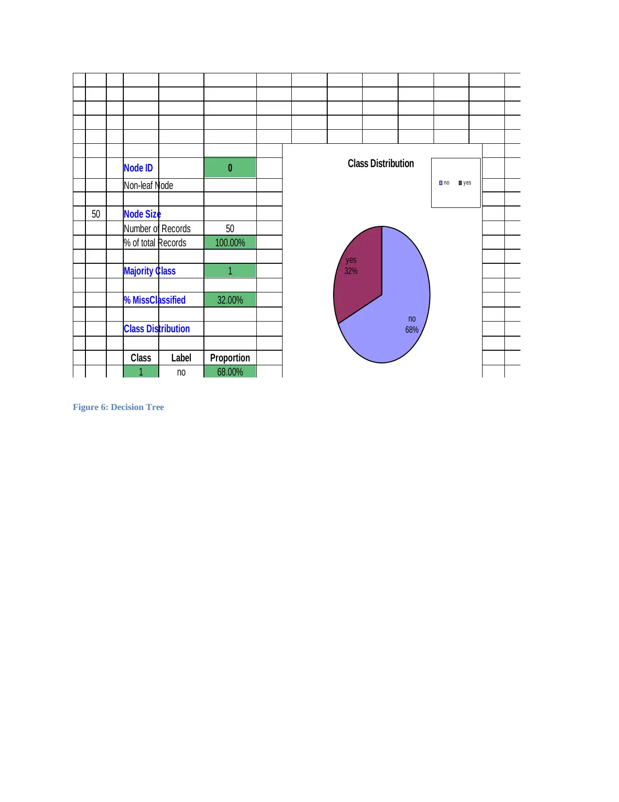
Figure 6: Decision Tree
Non-leaf Node
50 Node Size
Number of Records 50
% of total Records 100.00%
Majority Class 1
% MissClassified 32.00%
Class Distribution
Class Label Proportion
1 no 68.00%
no
68%
yes
32%
Class Distribution
no yes
Figure 6: Decision Tree
Paraphrase This Document
Need a fresh take? Get an instant paraphrase of this document with our AI Paraphraser
Rule Summary Table # Rules 2 8 Rule Text
Rule ID Class Length Support Confidence Capture Rule0 Playoff = no
0 no 0 100.0% 68.0% 100.0%
1 no 1 68.0% 100.0% 100.0% Rule1 IF Net Rating < 2.72
2 yes 1 32.0% 100.0% 100.0% THENPlayoff = no
Rule2 IF Net Rating >= 2.72
0 10 20 30 40 50 60
-1
0
1
2
3
How well do the Rules separate the Classes
Observations
Rule ID
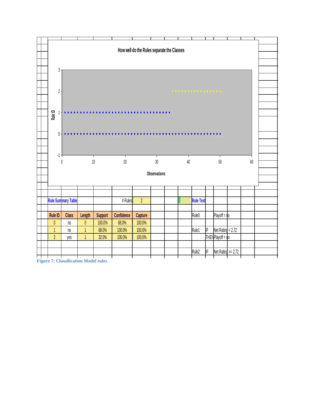
Figure 7: Classification Model rules
Rule ID Class Length Support Confidence Capture Rule0 Playoff = no
0 no 0 100.0% 68.0% 100.0%
1 no 1 68.0% 100.0% 100.0% Rule1 IF Net Rating < 2.72
2 yes 1 32.0% 100.0% 100.0% THENPlayoff = no
Rule2 IF Net Rating >= 2.72
0 10 20 30 40 50 60
-1
0
1
2
3
How well do the Rules separate the Classes
Observations
Rule ID
Figure 7: Classification Model rules
The model uses three rules to determine whether a team is in the playoffs or not. That is:
Rule 0; Playoff=No
Rule 1: If Net rating is less than 2.72, then a team is not included in the playoff
Rule 2: If Net rating is greater or equal to 2.72, then a team gets to the play offs.
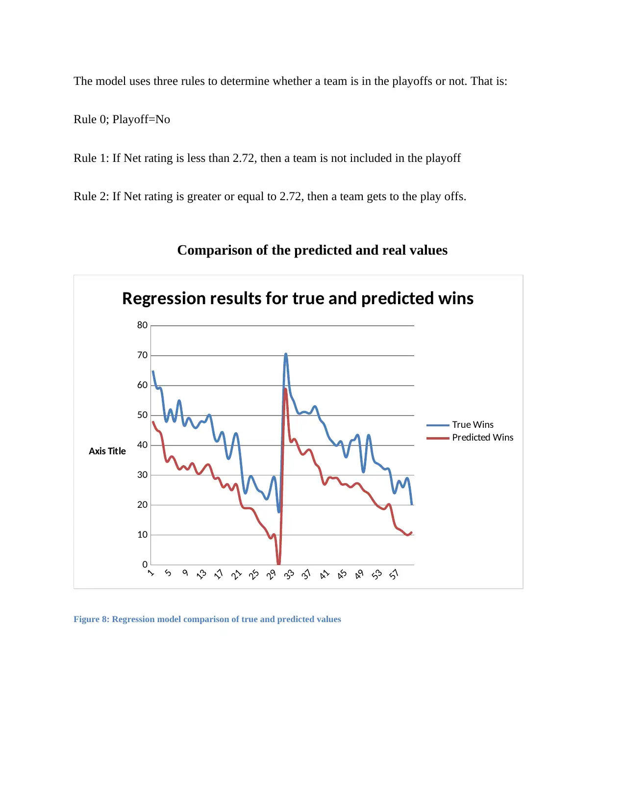
Comparison of the predicted and real values
1
5
9
13
17
21
25
29
33
37
41
45
49
53
57
0
10
20
30
40
50
60
70
80
Regression results for true and predicted wins
True Wins
Predicted Wins
Axis Title
Figure 8: Regression model comparison of true and predicted values
Rule 0; Playoff=No
Rule 1: If Net rating is less than 2.72, then a team is not included in the playoff
Rule 2: If Net rating is greater or equal to 2.72, then a team gets to the play offs.
Comparison of the predicted and real values
1
5
9
13
17
21
25
29
33
37
41
45
49
53
57
0
10
20
30
40
50
60
70
80
Regression results for true and predicted wins
True Wins
Predicted Wins
Axis Title
Figure 8: Regression model comparison of true and predicted values
⊘ This is a preview!⊘
Do you want full access?
Subscribe today to unlock all pages.
Trusted by 1+ million students worldwide
1 out of 14
Related Documents


Your All-in-One AI-Powered Toolkit for Academic Success.
+13062052269
info@desklib.com
Available 24*7 on WhatsApp / Email
![[object Object]](/_next/static/media/star-bottom.7253800d.svg)
Unlock your academic potential
Copyright © 2020–2026 A2Z Services. All Rights Reserved. Developed and managed by ZUCOL.