Advanced Robotics Project 2 - Neural Networks for Robot Control Report

This project report details the implementation of neural networks for robot control using SIMULINK. The project begins with the development of a SIMULINK model based on dynamic equations of a two-link robot, which accepts driving torques and generates joint positions and velocities. A computed-torque controller (CTC) is then implemented in SIMULINK. The core of the project involves using a neural network controller (NNC) to perform the CTC, with the NN controller also implemented in SIMULINK. The report includes the CTC equations and methods, the implementation of CTC and NNC in the simulations, and the NN structure. It presents the results of the CTC controller gains with comparison errors and the NNC training results. The project aims to demonstrate the effectiveness of the developed controllers through simulation and analysis of the robot's performance under different control schemes, including the performance comparison of the CTC and NNC methods and the evaluation of the accuracy of the outcomes. The simulation results include waveforms of the training data and the robot arm movements.

1NEUTRAL NETWORKS FOR ROBOTIC CONTROL
Neutral Networks for Robotic Control
Name
Professor/Tutor
Date
Institution

2NEUTRAL NETWORKS FOR ROBOTIC CONTROL
Introduction
To this day, many scholars pay more and more attention to the problem of controlling robots to have a
restricted movement (Cui, et al., 2013). Generally, there is existence of constraints on the input and the
output of the robot system, like the dead-zone, safety specification, and saturation (Liu & Tong, 2016).
Uncertainties in the robot control manipulator that interact with humans and environment poses a
challenge since it has some dynamics and disturbances that are unknown. In the recent past, more
researchers and scholars a like have used the adaptive neutral for suitable schemes of control for the
systems that are nonlinear (Cheng, et al., 2009). Yet some researchers have used adaptive Jacobian
scheme for the approximation of unknown schemes of kinematics for the manipulator. There are some
who have used radial basis function of neutral network for the compensation of the non linear terms that
have seem to be complicated closed-loop dynamics of the robot systems. Another control scheme was
devised based on neutral network for the nonlinear systems of affine which are aligned to the constraints
and have a discrete time (Cheng, et al., 2012).
Robot trajectory planning is the most basic element in robotics applications and generally automation.
Generation of trajectories that has some specific features is an important point that ensures some
important results are achieved regarding the quality and an easy performance needed for the motion,
especially when the speeds of operation are high to necessitate any application (Gasparetto, et al.,
2012). The robot trajectory is divided into two categories, the joint space and the cartesian-space
trajectories. The joint space trajectory planning, like the polynomials spline and time-optimal methods.
Joint space trajectory planning is commonly used in robotics for a continuous, and a smooth motion
from the one set of n joint angles to the other, for example when there’s a movement between two
separate cartesian poses where the reversed pose solution yielded two different sets of n joint angles.
The joint-space trajectory generation happens at run time for all n joints simultaneously and
independently. Cartesian trajectory planning are trajectories that passes through specific points, knot
points in b-splines. They can also pass through some straight-line paths that are connected through
points. The position and the orientations must be interpolated.
This paper is aimed at using dynamic equations to build a SIMULINK model of the robot that can
accepts the driving torques in robots’ joints and generates positions and velocities of the joints of the
robots. There shall also be a computed-torque controller (CTC) which shall also be done by SIMULINK
for the same robot, and the use of neutral network (NNC) to be able to perform the CTC and implement
the NN controller in SIMULINK. There shall be CTC equations and methods, and CTC implementation
in the simulations, the NNC methods including the NN structure. Then analysis of the results of the
CTC controller gains with comparison errors and NNC training results and check the accuracy of the
outcomes.
Simulation Model of the Robot.
Simulation is a method of designing, executing the model and analyzing the implementation output of a
real or theoretical physical arrangement. Simulation is indeed very prevalent in life; it allows to compre
hend reality and its complexity. In robotics, simulations have some various ways, and with different
software which majorly focuses on the motion of the robot and manipulating it when certain commands
are applied to it or set to act in different environment. Motion simulation have a central role to play

3NEUTRAL NETWORKS FOR ROBOTIC CONTROL
among all simulations, they include kinematics or what is known as dynamic models of the robotic
manipulators. The type of models used shall depend on the aim of the simulation system. For instance,
when using the trajectory planning algorithms, they rely on the kinematic models. On a similar fashion,
the development of a cell of a robot is simulated effectively using kinematic model only. Modelling and
simulating a robotic manipulator technique are different and possible. The only difference is the way the
user uses their model. When applying a block diagram simulator, it requires combination of the blocks
and describing the system, and some requires manual coding. When the system is very complex, it more
often brings a lot of issues and overcoming these issues there are techniques and approaches that exist to
automatically develop the kinematic and dynamic model of the robot. The tools used for simulating
robots can be categorized into two: tools that can simulate systems generally, and special tools made
only for robot modelling. The tools that does simulation generally have special user interfaces or
modules and libraries that simplifies the robot development and the environment to which the robot
operate on. The merit of such integrated toolbox is their flexibility to allow you to use other available
tools for the simulation to do other different tasks (Kumar & Narayan, 2011). A case of such is the
design system that allows you to design a control system, study the simulation, and see the results. The
major tool of this kind is MATLAB/Simulink, others are Mathematica, Dymola/Modelica etc.
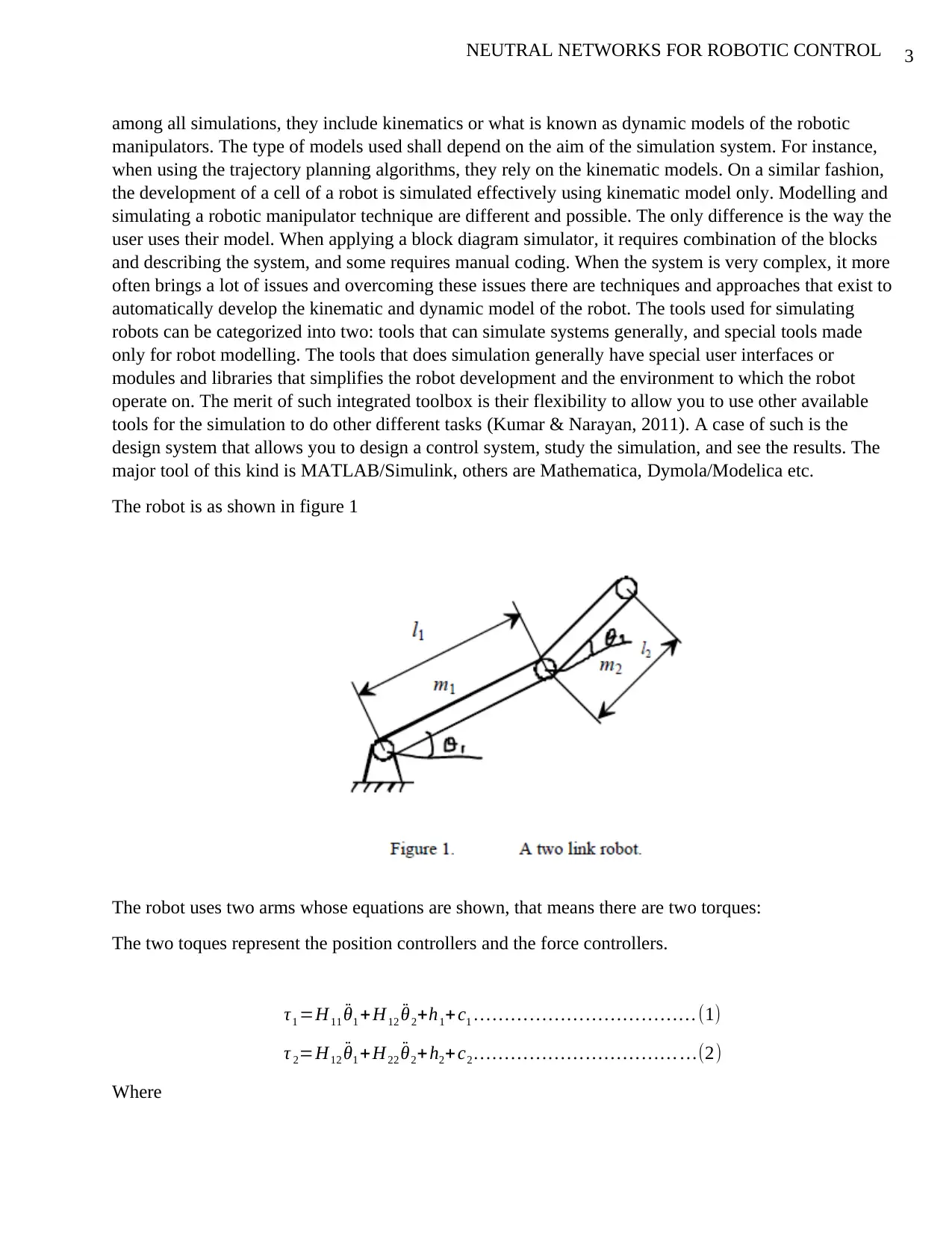
The robot is as shown in figure 1
The robot uses two arms whose equations are shown, that means there are two torques:
The two toques represent the position controllers and the force controllers.
τ1 =H11 ¨θ1 + H12 ¨θ2+h1+ c1 … … … … … … … … … … … … (1)
τ 2=H12 ¨θ1 + H22 ¨θ2+ h2+ c2 … … … … … … … … … … … …(2)
Where

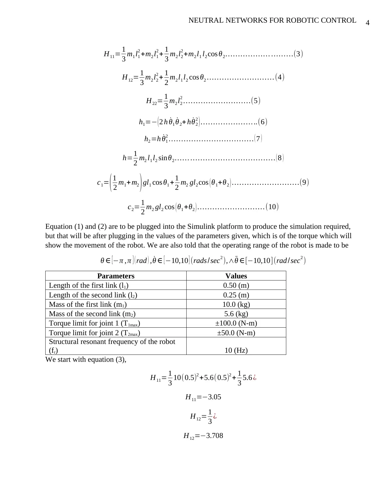
4NEUTRAL NETWORKS FOR ROBOTIC CONTROL
H11= 1
3 m1 l1
2 +m2 l1
2 + 1
3 m2 l2
2 +m2 l1 l2 cos θ2 … … … … … … … … …(3)
H12= 1
3 m2 l2
2 + 1
2 m2 l1 l2 cos θ2 … … … … … … … … … (4)
H22= 1
3 m2 l2
2 … … … … … … … … …(5)
h1=− ( 2 h ˙θ1 ˙θ2+ h ˙θ2
2 ) … … … … … … … ..(6)
h2 =h ˙θ1
2 … … … … … … … … … … … . ( 7 )
h=1
2 m2 l1 l2 sinθ2 … … … … … … … … … … … … … . ( 8 )
c1= ( 1
2 m1+m2 ) gl1 cos θ1 +1
2 m2 gl2 cos ( θ1+θ2 ) … … … … … … … … …(9)
c2= 1
2 m2 gl2 cos ( θ1 +θ2 ) … … … … … … … … … (10)
Equation (1) and (2) are to be plugged into the Simulink platform to produce the simulation required,
but that will be after plugging in the values of the parameters given, which is of the torque which will
show the movement of the robot. We are also told that the operating range of the robot is made to be
θ ∈ [−π , π ] ( rad ) , ˙θ ∈ [−10,10 ] (rads /sec2 ),∧ ¨θ ∈[−10,10](rad /sec2 )
Parameters Values
Length of the first link (l1) 0.50 (m)
Length of the second link (l2) 0.25 (m)
Mass of the first link (m1) 10.0 (kg)
Mass of the second link (m2) 5.6 (kg)
Torque limit for joint 1 (T1max) ±100.0 (N-m)
Torque limit for joint 2 (T2max) ±50.0 (N-m)
Structural resonant frequency of the robot
(fr) 10 (Hz)
We start with equation (3),
H11= 1
3 10(0.5)2 +5.6(0.5)2 + 1
3 5.6 ¿
H11=−3.05
H12= 1
3 ¿
H12=−3.708

5NEUTRAL NETWORKS FOR ROBOTIC CONTROL
H22= 1
3 (5.6)¿
h=0
c1=5.3 gcos θ1 +0.7 g cos ( θ1+θ2 )
c2=0.7 g
h1=0
h2 =0
Therefore
τ1 =3.05+37.08+5.3 g +0.7 g=40.13+6 g
τ1 =40.13+6 g
And
τ 2=0.7 g−35.91
Now we need to construct a neutral network that produces the calculation of the following equations:
We have replaced the ¨θ1=x1; ¨θ2= x2;
y1=H11 ¨θ1+ H12 ¨θ2 +c1
y2=H21 ¨θ1+ H22 ¨θ2 +c2
With the parameters as shown below:
θ ∈ [−π , π ] ( rad ) , ˙θ ∈ [−10,10 ] (rads /sec2 ),∧ ¨θ ∈[−10,10](rad /sec2 )
The code that follows the equations shall be as follows
% =========
% Clear the workspace
% =========
clear all
close all
clc
Numd=1000;
% ==============
% Generating training paterns

6NEUTRAL NETWORKS FOR ROBOTIC CONTROL
% ==============
% Generate 200 random inputs x1 =[-10 10]
H11=-3.05;
H12=-3.708;
H22=0.117;
x1=12*rand(1,Numd)-6;
% Generate 200 random inputs for x2=[-10 10]
x2=2.4*rand(1,Numd)-1.2;
% Generate outputs according to equations
y1=H11(x1)+H12(x2);
%+(5*rand(1,Numd)2.5);
y2=H12(x1)+ H22(x2);
%+(5*rand(1,Numd)2.5);
% ==============
% Construct the NN
% ==============
% For a quick help in Neural network toolbox, you can type 'help
% nnet' in MATLAB command window for a list of available commands to
use
% in the NN toolbox.
% Initialise the Neural Network. the NN initialisation is
feedforwardnet
% type 'help feedforwardnet' in MATLAB command window for help.
net=feedforwardnet([10,5]); % two hidden layers with 10 and 5 neurons
in each
% Set training parameters
net.trainParam.show=50;
net.trainParam.lr=0.05;
net.trainParam.mc=0.95;
net.trainParam.epochs=1000;
net.trainParam.goal=1e-10;
net.trainParam.max_fail=20;
% validation check counts
% ==============
% Start training the NN
% ==============
net=train(net,[x1;x2],[y1;y2]);
% ==============
% Save the training results
% ==============
save step1 net
% ==============
% Test the training results on 20 randomly generated points
% ==============
x1t=12*rand(1,20)-6;
x2t=2.4*rand(1,20)-1.2;
y1t=H11(x1)+H12(x2);

7NEUTRAL NETWORKS FOR ROBOTIC CONTROL
y2t=H12(x1)+H22(x2);
a=sim(net,[x1t;x2t]);
figure(1)
subplot(211)
hold off
plot(a(1,:),'k-o','LineWidth', 1);
hold on
plot(y1t,'r-+','LineWidth',1);
hold off
legend('NN output', 'equation for Y1')
grid
title('NN performance after 1000 iterations')
subplot(212)
hold off
plot(a(2,:),'k-o','LineWidth', 1);
hold on
plot(y2t,'r-+','LineWidth',1);
hold off
legend('NN output', 'equation for Y2')
grid
figure(2)
error1=y1t-a(1,:);
error2=y2t-a(2,:);
hold off
plot(error1,'k','LineWidth',1)
hold on
plot(error2,'r','LineWidth',1);
legend('Y1 error', 'Y2 error')
title('NN prediction error after 1000 iterations')
grid
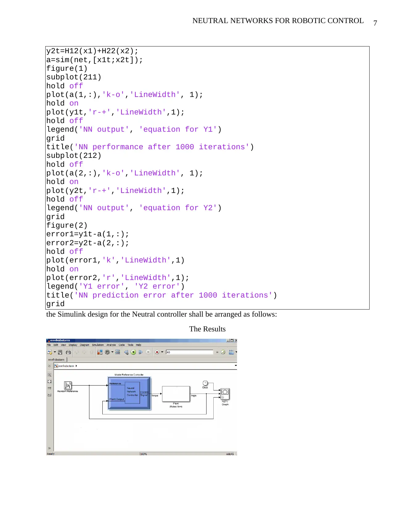
the Simulink design for the Neutral controller shall be arranged as follows:
The Results

8NEUTRAL NETWORKS FOR ROBOTIC CONTROL
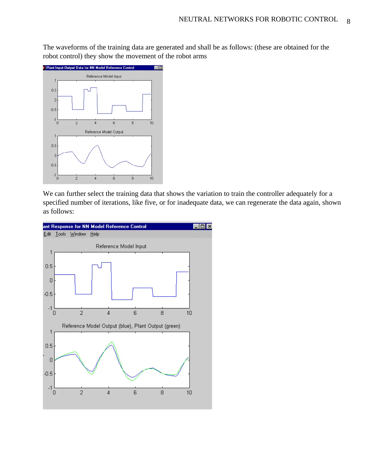
The waveforms of the training data are generated and shall be as follows: (these are obtained for the
robot control) they show the movement of the robot arms
We can further select the training data that shows the variation to train the controller adequately for a
specified number of iterations, like five, or for inadequate data, we can regenerate the data again, shown
as follows:

9NEUTRAL NETWORKS FOR ROBOTIC CONTROL
The upper axis shows the random input reference used in the training, and the lower axis shows the
reference response of the model and the closed loop plant, the response of the plant is to follow the
reference model.
Computed Torque Controller
Is a prolific non linear controller vastly applied in robotics manipulator. CTC is a feedback-linear
technique that needs a computed torque of the arm by what is known as a non linear law of control. The
controller works well when the physical and dynamic parameters, however, the manipulator part of the
robot is varied in the dynamic parameters, in this condition there’s no acceptable performance of the
controller (Vidyasagar & Spong , 2009). Ideally, many systems that are physical, like the manipulation
of robots, the parameters like the time variants are not known, this is now where CTC can be used for
compensation of the robot manipulator dynamic equation. There’s an ever-growing research of CTC
and the application of the robot manipulator reported in (Siciliano & Khatib, 2018). There has been a
functional predictive controller proposed that can be used instead of the CTC in case there’s a need to
track a response in an environment that is uncertain. Nonetheless, the two controllers can and have been
used a linear feedback mechanism, though in a predictive manner that results in a better performance.
CTC that has a parametric model regression is presented and used in an arm of a robot (Nguyen-Tuong,
et al., 2018). The controller in question can pose a problem when the dynamic model is uncertain. Based
on different analyses, CTC is an important nonlinear controller to some systems based on the linearized
feedback and computes the arm torques which are required by a use of non linear control law. However,
when physical and dynamic parameters can be identified the controller works very well; ideally large
amount of systems have misgivings and the controller in sliding mode curbs these challenges posed.
Computed Torque Formulation applied to robot arm
The main idea why CTC is used is to linearize the feedback. Initially the algorithm was referred to as
feedback linearization technique. The working principle is that it assumes that the intended motion
trajectory for the manipulator qt (t ), is found out by the path planner. It defines the error of tracking as:
e ( t ) =qd ( t ) −qa ( t ) … … … … … … … … … .(11)
Where: e (t) is the plant error, qd (t ) is the variable input desired in the system qa (t) is the real
displacement. The equivalent equation of the linear state-space, which is in the form of x= A x +B U is
written as:
x= [0 1
0 0 ]x + [0
1 ]U … … … … … … … … … … … … … .(12)
When the torque equations are as follows:
τ1 =H11 ¨θ1 + H12 ¨θ2+h1+ c1
τ 2=H12 ¨θ1 + H22 ¨θ2+ h2+ c2
[ T1
T2 ] =
[ H11 H12
H21 H22 ] [ ¨θ1
¨θ2 ] + [ h1
h2 ] + [ c1
c2 ] … … … … … … … (13)

10NEUTRAL NETWORKS FOR ROBOTIC CONTROL
We have now obtained the values of H11 , H12 , H22 ,h1∧h2 the values of the ¨θ1∧ ¨θ2 are accelerations for
the joints of the robot. The CTC equation will therefore be:
τ c=
[ H11 H12
H12 H22 ] [ ¨θ1
d + K v 1 ( ˙θ1
d − ˙θ1 ) + K p 1 (θ1
d−θ1)
¨θ2
d + K v 2 ( ˙θ2
d − ˙θ2 ) + K p 2 (θ2
d−θ2) ] + [ h1
h2 ] +
[ c1
c2 ] … … … … …( 14)
The superscript d represents the desired accelerations, velocities and positions; while
K p 1 , K p2 , Kv 1 ,∧Kv 2 are control gains that can be calculated using the following characteristics of a
second order system:
¨e + Kv ˙e+K p e=0 … … … … … … … … … ( 15 )
Therefore, to achieve the certain damping ratio ζ (≥1)and a natural frequency ωn (≤ 0.5 ωn ),
Kv =2 ζ ωn∧K p=ωn
2 … … … … … … …..(16)
The parameters of the variables are given as follows; ζ =1 ,∧ωn=0.5 ωn the gains can be determined.
Discussion
Conclusion
References
Cheng, L., Hou, Z.-G. & Tan, M., 2009. Adaptive neutral network tracking control for manipulators
with uncertain kinematics,dynamics and actuator model. Automatica, Volume 10, pp. 2312-
2318.

11NEUTRAL NETWORKS FOR ROBOTIC CONTROL
Cheng, L., Hou, Z.-G., Tan, M. & Zhang, W.-J., 2012. Tracking control of a closed-chain five-bar robot
with two degrees of freedom by integration of an approximation-based approach and
mechanical design. IEEE Transactions on Systems, Man, and Cybernetics, Part B
(Cybernetics),, 5(45), pp. 1470-1479.
Cui, R., Guo, J. & Gao, B., 2013. Game theory-based nego-tiation for multiple robots task allocation.
Robotica, 06(31), pp. 923-934.
Gasparetto, A., Boscariol, P., Lanzutti, A. & Vidoni, R., 2012. Trajectory Planning in Robotics.
Mathematics in Computer Science, 6(3), pp. 269-279.
Kumar, N. P. & Narayan, S. Y., 2011. Simulation in Robotics. RECENT ADVANCES IN
MANUFACTURING ENGINEERING & TECHNOLOGY, pp. 2-5.
Liu, Y.-J. & Tong, S., 2016. Barrier lyapunov functions-based adaptive control for a class of nonlinear
pure-feedback systems with full state constraints. Automatica, Volume 64, pp. 70-75.
Nguyen-Tuong, D., Seeger , M. & Peters, J., 2018. Computed torque control with nonparametric
regression models. s.l., IEEE conference proceeding.
Siciliano, B. & Khatib, O., 2018. Springer handbook of robotics: , New York-USA: Springer-Verlag.
Vidyasagar, M. & Spong , M. W., 2009. Robot dynamics and control, Wiley-India: Wiley.