Birkbeck Spring 2018: NLSY79 Data Analysis in Business Research
VerifiedAdded on 2023/06/14
|23
|5140
|80
Homework Assignment
AI Summary
This assignment presents a detailed statistical analysis of the National Longitudinal Survey of Youth 1979 (NLSY79) data, conducted for the Statistical Methods for Business Research course at Birkbeck, Spring 2018. The analysis includes descriptive statistics, such as mean, standard deviation, and percentile calculations for variables like age, earnings, and education. Inferential statistics involve t-tests to compare earnings across different groups (e.g., poverty status), Chi-Square tests to assess associations between education and divorce, and correlation analyses using both Pearson and Spearman coefficients. The assignment also covers multiple regression models, examining the impact of various factors on earnings, and addresses potential issues like omitted variables, heteroscedasticity, and multicollinearity. The do-file codes are provided in the appendix.
Statistical Methods for Business Research
Department of Management, Birkbeck
Coursework Spring 2018
Student Name:
ID:
Date: 18th March 2018
Department of Management, Birkbeck
Coursework Spring 2018
Student Name:
ID:
Date: 18th March 2018
Paraphrase This Document
Need a fresh take? Get an instant paraphrase of this document with our AI Paraphraser
Questions Descriptive and Inferential Statistics
Question 1
In STATA; codes provided in the appendix
Question 2
In STATA; codes provided in the appendix
Question 3
In STATA; codes provided in the appendix
Question 4
HOURS 540 40.53519 9.114845 10 60
S 540 13.52778 2.40384 6 20
EARNINGS 540 19.05415 14.18551 2.25 134.61
MALE 540 .5 .5004636 0 1
AGE 540 40.83333 2.18402 37 45
Variable Obs Mean Std. Dev. Min Max
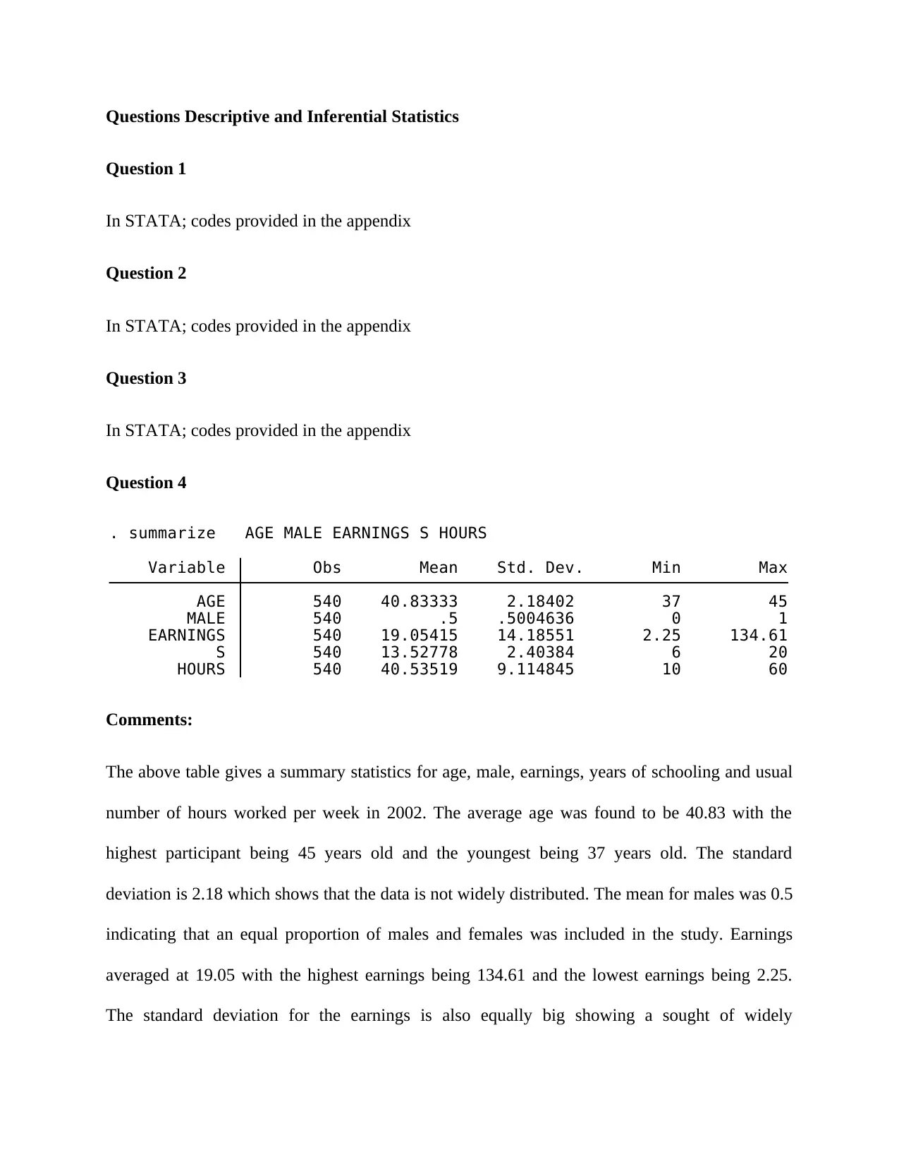
. summarize AGE MALE EARNINGS S HOURS
Comments:
The above table gives a summary statistics for age, male, earnings, years of schooling and usual
number of hours worked per week in 2002. The average age was found to be 40.83 with the
highest participant being 45 years old and the youngest being 37 years old. The standard
deviation is 2.18 which shows that the data is not widely distributed. The mean for males was 0.5
indicating that an equal proportion of males and females was included in the study. Earnings
averaged at 19.05 with the highest earnings being 134.61 and the lowest earnings being 2.25.
The standard deviation for the earnings is also equally big showing a sought of widely
Question 1
In STATA; codes provided in the appendix
Question 2
In STATA; codes provided in the appendix
Question 3
In STATA; codes provided in the appendix
Question 4
HOURS 540 40.53519 9.114845 10 60
S 540 13.52778 2.40384 6 20
EARNINGS 540 19.05415 14.18551 2.25 134.61
MALE 540 .5 .5004636 0 1
AGE 540 40.83333 2.18402 37 45
Variable Obs Mean Std. Dev. Min Max
. summarize AGE MALE EARNINGS S HOURS
Comments:
The above table gives a summary statistics for age, male, earnings, years of schooling and usual
number of hours worked per week in 2002. The average age was found to be 40.83 with the
highest participant being 45 years old and the youngest being 37 years old. The standard
deviation is 2.18 which shows that the data is not widely distributed. The mean for males was 0.5
indicating that an equal proportion of males and females was included in the study. Earnings
averaged at 19.05 with the highest earnings being 134.61 and the lowest earnings being 2.25.
The standard deviation for the earnings is also equally big showing a sought of widely
distributed dataset. The average years of schooling was 13.53 with the least number of schooling
and the highest number of schooling years being 6 and 20 respectively. The mean usual number
of hours worked per week in 2002 was 40.54 with the highest usual number of hours of work per
week being 60 while the lowest being 10 hours a week.
Question 5:
75 16 15 16
50 12.5 12 13
S 540 25 12 12 12
75 42.75 42 43
50 41 40 41
AGE 540 25 39 39 39
75 20.40385 20.03846 20.74951
50 18.01923 17.3931 18.55769
EXP 540 25 14.85096 14.34615 15.42308
Variable Obs Percentile Centile [95% Conf. Interval]
Binom. Interp.
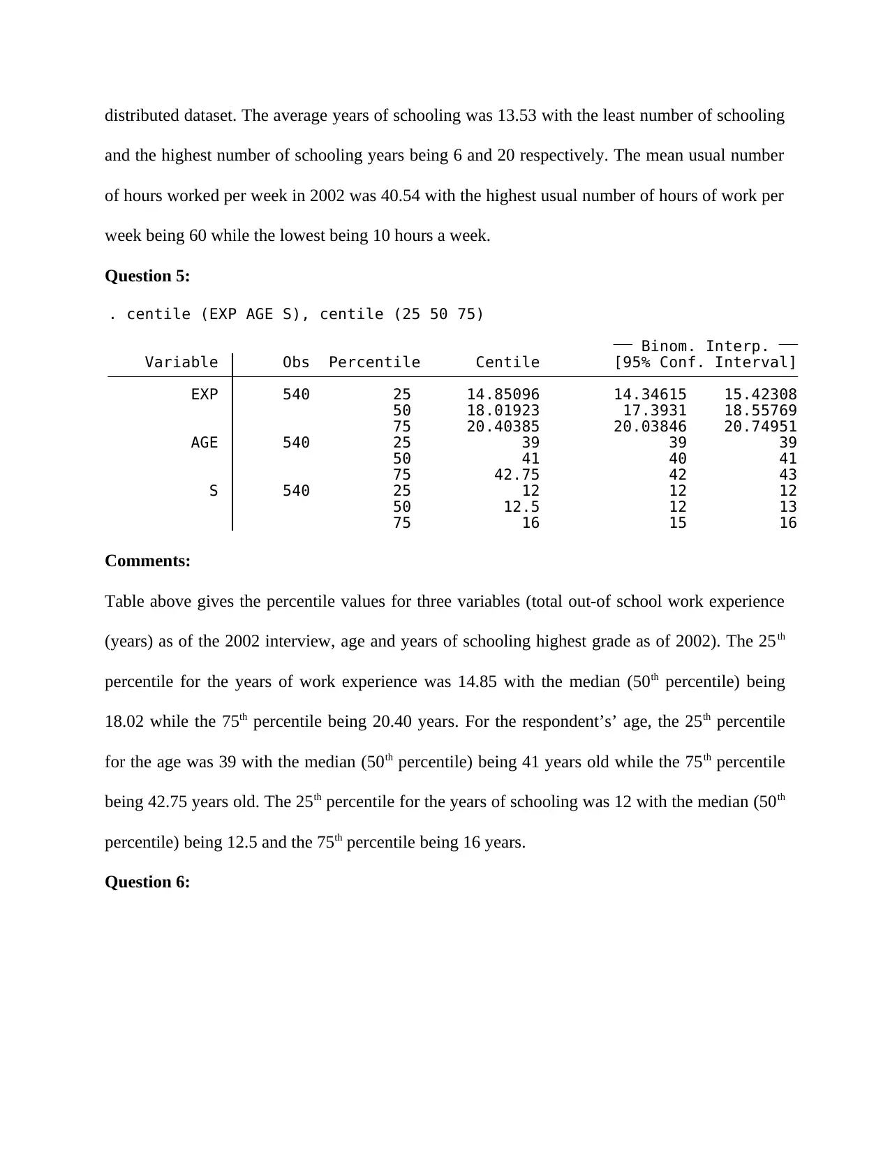
. centile (EXP AGE S), centile (25 50 75)
Comments:
Table above gives the percentile values for three variables (total out-of school work experience
(years) as of the 2002 interview, age and years of schooling highest grade as of 2002). The 25th
percentile for the years of work experience was 14.85 with the median (50th percentile) being
18.02 while the 75th percentile being 20.40 years. For the respondent’s’ age, the 25th percentile
for the age was 39 with the median (50th percentile) being 41 years old while the 75th percentile
being 42.75 years old. The 25th percentile for the years of schooling was 12 with the median (50th
percentile) being 12.5 and the 75th percentile being 16 years.
Question 6:
and the highest number of schooling years being 6 and 20 respectively. The mean usual number
of hours worked per week in 2002 was 40.54 with the highest usual number of hours of work per
week being 60 while the lowest being 10 hours a week.
Question 5:
75 16 15 16
50 12.5 12 13
S 540 25 12 12 12
75 42.75 42 43
50 41 40 41
AGE 540 25 39 39 39
75 20.40385 20.03846 20.74951
50 18.01923 17.3931 18.55769
EXP 540 25 14.85096 14.34615 15.42308
Variable Obs Percentile Centile [95% Conf. Interval]
Binom. Interp.
. centile (EXP AGE S), centile (25 50 75)
Comments:
Table above gives the percentile values for three variables (total out-of school work experience
(years) as of the 2002 interview, age and years of schooling highest grade as of 2002). The 25th
percentile for the years of work experience was 14.85 with the median (50th percentile) being
18.02 while the 75th percentile being 20.40 years. For the respondent’s’ age, the 25th percentile
for the age was 39 with the median (50th percentile) being 41 years old while the 75th percentile
being 42.75 years old. The 25th percentile for the years of schooling was 12 with the median (50th
percentile) being 12.5 and the 75th percentile being 16 years.
Question 6:
⊘ This is a preview!⊘
Do you want full access?
Subscribe today to unlock all pages.
Trusted by 1+ million students worldwide
Pr(T < t) = 0.7799 Pr(|T| > |t|) = 0.4402 Pr(T > t) = 0.2201
Ha: diff < 0 Ha: diff != 0 Ha: diff > 0
Ho: diff = 0 degrees of freedom = 507
diff = mean(0) - mean(1) t = 0.7724
diff 1.431688 1.85348 -2.20976 5.073136
combined 509 19.09014 .6224029 14.04205 17.86734 20.31294
1 66 17.84409 1.700428 13.81434 14.4481 21.24008
0 443 19.27578 .6690373 14.08161 17.96089 20.59067
Group Obs Mean Std. Err. Std. Dev. [95% Conf. Interval]
Two-sample t test with equal variances
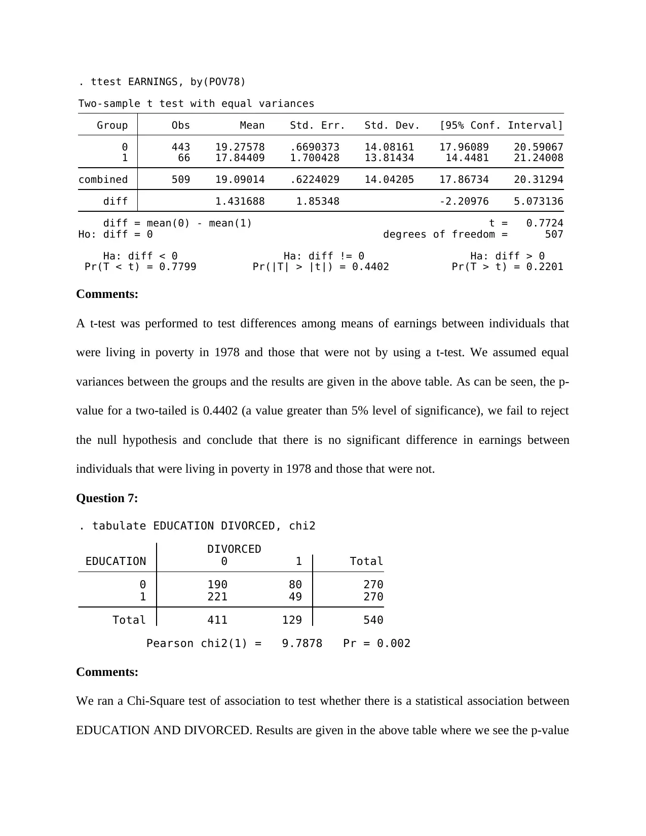
. ttest EARNINGS, by(POV78)
Comments:
A t-test was performed to test differences among means of earnings between individuals that
were living in poverty in 1978 and those that were not by using a t-test. We assumed equal
variances between the groups and the results are given in the above table. As can be seen, the p-
value for a two-tailed is 0.4402 (a value greater than 5% level of significance), we fail to reject
the null hypothesis and conclude that there is no significant difference in earnings between
individuals that were living in poverty in 1978 and those that were not.
Question 7:
Pearson chi2(1) = 9.7878 Pr = 0.002
Total 411 129 540
1 221 49 270
0 190 80 270
EDUCATION 0 1 Total
DIVORCED
. tabulate EDUCATION DIVORCED, chi2
Comments:
We ran a Chi-Square test of association to test whether there is a statistical association between
EDUCATION AND DIVORCED. Results are given in the above table where we see the p-value
Ha: diff < 0 Ha: diff != 0 Ha: diff > 0
Ho: diff = 0 degrees of freedom = 507
diff = mean(0) - mean(1) t = 0.7724
diff 1.431688 1.85348 -2.20976 5.073136
combined 509 19.09014 .6224029 14.04205 17.86734 20.31294
1 66 17.84409 1.700428 13.81434 14.4481 21.24008
0 443 19.27578 .6690373 14.08161 17.96089 20.59067
Group Obs Mean Std. Err. Std. Dev. [95% Conf. Interval]
Two-sample t test with equal variances
. ttest EARNINGS, by(POV78)
Comments:
A t-test was performed to test differences among means of earnings between individuals that
were living in poverty in 1978 and those that were not by using a t-test. We assumed equal
variances between the groups and the results are given in the above table. As can be seen, the p-
value for a two-tailed is 0.4402 (a value greater than 5% level of significance), we fail to reject
the null hypothesis and conclude that there is no significant difference in earnings between
individuals that were living in poverty in 1978 and those that were not.
Question 7:
Pearson chi2(1) = 9.7878 Pr = 0.002
Total 411 129 540
1 221 49 270
0 190 80 270
EDUCATION 0 1 Total
DIVORCED
. tabulate EDUCATION DIVORCED, chi2
Comments:
We ran a Chi-Square test of association to test whether there is a statistical association between
EDUCATION AND DIVORCED. Results are given in the above table where we see the p-value
Paraphrase This Document
Need a fresh take? Get an instant paraphrase of this document with our AI Paraphraser
to be 0.002 (a value less than 5% significance level), we therefore reject the null hypothesis and
conclude that there is strong evidence of significant association between EDUCATION and
DIVORCED.
Question 8:
0.0000 0.0000
SIBLINGS -0.3344 -0.3214 1.0000
0.0000
SF 0.6364 1.0000
SM 1.0000
SM SF SIBLINGS
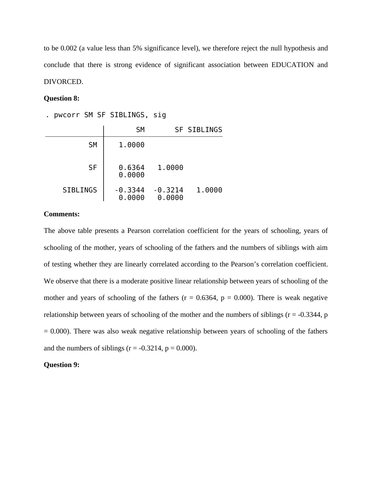
. pwcorr SM SF SIBLINGS, sig
Comments:
The above table presents a Pearson correlation coefficient for the years of schooling, years of
schooling of the mother, years of schooling of the fathers and the numbers of siblings with aim
of testing whether they are linearly correlated according to the Pearson’s correlation coefficient.
We observe that there is a moderate positive linear relationship between years of schooling of the
mother and years of schooling of the fathers (r = 0.6364, p = 0.000). There is weak negative
relationship between years of schooling of the mother and the numbers of siblings (r = -0.3344, p
= 0.000). There was also weak negative relationship between years of schooling of the fathers
and the numbers of siblings (r = -0.3214, p = 0.000).
Question 9:
conclude that there is strong evidence of significant association between EDUCATION and
DIVORCED.
Question 8:
0.0000 0.0000
SIBLINGS -0.3344 -0.3214 1.0000
0.0000
SF 0.6364 1.0000
SM 1.0000
SM SF SIBLINGS
. pwcorr SM SF SIBLINGS, sig
Comments:
The above table presents a Pearson correlation coefficient for the years of schooling, years of
schooling of the mother, years of schooling of the fathers and the numbers of siblings with aim
of testing whether they are linearly correlated according to the Pearson’s correlation coefficient.
We observe that there is a moderate positive linear relationship between years of schooling of the
mother and years of schooling of the fathers (r = 0.6364, p = 0.000). There is weak negative
relationship between years of schooling of the mother and the numbers of siblings (r = -0.3344, p
= 0.000). There was also weak negative relationship between years of schooling of the fathers
and the numbers of siblings (r = -0.3214, p = 0.000).
Question 9:
0.0000 0.0000
SIBLINGS -0.2874 -0.2524 1.0000
0.0000
SF 0.5998 1.0000
SM 1.0000
SM SF SIBLINGS
Sig. level
rho
Key
(obs=540)
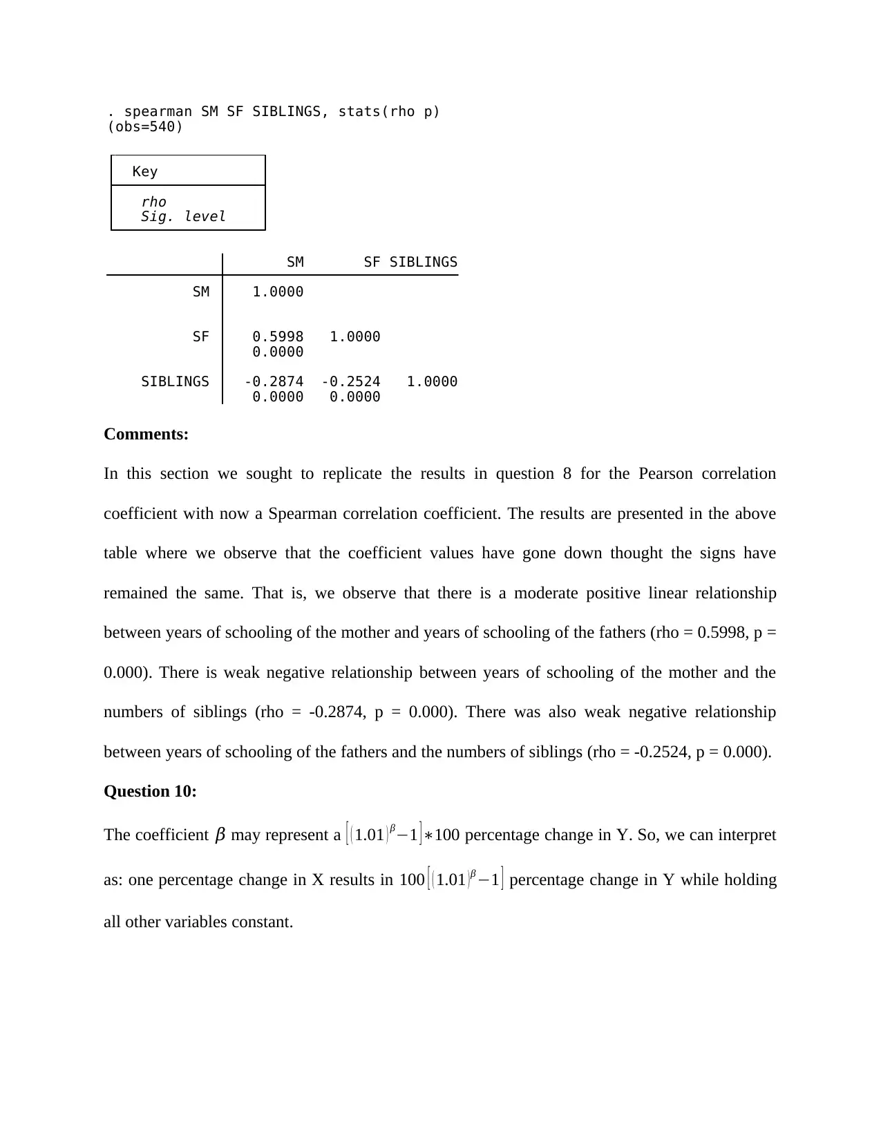
. spearman SM SF SIBLINGS, stats(rho p)
Comments:
In this section we sought to replicate the results in question 8 for the Pearson correlation
coefficient with now a Spearman correlation coefficient. The results are presented in the above
table where we observe that the coefficient values have gone down thought the signs have
remained the same. That is, we observe that there is a moderate positive linear relationship
between years of schooling of the mother and years of schooling of the fathers (rho = 0.5998, p =
0.000). There is weak negative relationship between years of schooling of the mother and the
numbers of siblings (rho = -0.2874, p = 0.000). There was also weak negative relationship
between years of schooling of the fathers and the numbers of siblings (rho = -0.2524, p = 0.000).
Question 10:
The coefficient 𝛽 may represent a [ ( 1.01 ) β−1 ] ∗100 percentage change in Y. So, we can interpret
as: one percentage change in X results in 100 [ ( 1.01 )β −1 ] percentage change in Y while holding
all other variables constant.
SIBLINGS -0.2874 -0.2524 1.0000
0.0000
SF 0.5998 1.0000
SM 1.0000
SM SF SIBLINGS
Sig. level
rho
Key
(obs=540)
. spearman SM SF SIBLINGS, stats(rho p)
Comments:
In this section we sought to replicate the results in question 8 for the Pearson correlation
coefficient with now a Spearman correlation coefficient. The results are presented in the above
table where we observe that the coefficient values have gone down thought the signs have
remained the same. That is, we observe that there is a moderate positive linear relationship
between years of schooling of the mother and years of schooling of the fathers (rho = 0.5998, p =
0.000). There is weak negative relationship between years of schooling of the mother and the
numbers of siblings (rho = -0.2874, p = 0.000). There was also weak negative relationship
between years of schooling of the fathers and the numbers of siblings (rho = -0.2524, p = 0.000).
Question 10:
The coefficient 𝛽 may represent a [ ( 1.01 ) β−1 ] ∗100 percentage change in Y. So, we can interpret
as: one percentage change in X results in 100 [ ( 1.01 )β −1 ] percentage change in Y while holding
all other variables constant.
⊘ This is a preview!⊘
Do you want full access?
Subscribe today to unlock all pages.
Trusted by 1+ million students worldwide
Multiple Regressions, Dummy Variables and Logistic Regressions
Question 1:
a)
Model 1
_cons .7084384 .4674146 1.52 0.130 -.209887 1.626764
POV78 .0239272 .0754117 0.32 0.751 -.1242336 .1720879
ETHWHITE .0969069 .0690004 1.40 0.161 -.0386576 .2324714
MALE .2406604 .0477641 5.04 0.000 .1468187 .3345021
S .1157567 .0100961 11.47 0.000 .095921 .1355924
AGE .0067992 .0109194 0.62 0.534 -.014654 .0282524
InEARNINGS Coef. Std. Err. t P>|t| [95% Conf. Interval]
Total 193.225204 508 .380364575 Root MSE = .5383
Adj R-squared = 0.2382
Residual 145.75335 503 .289768091 R-squared = 0.2457
Model 47.4718541 5 9.49437081 Prob > F = 0.0000
F( 5, 503) = 32.77
Source SS df MS Number of obs = 509
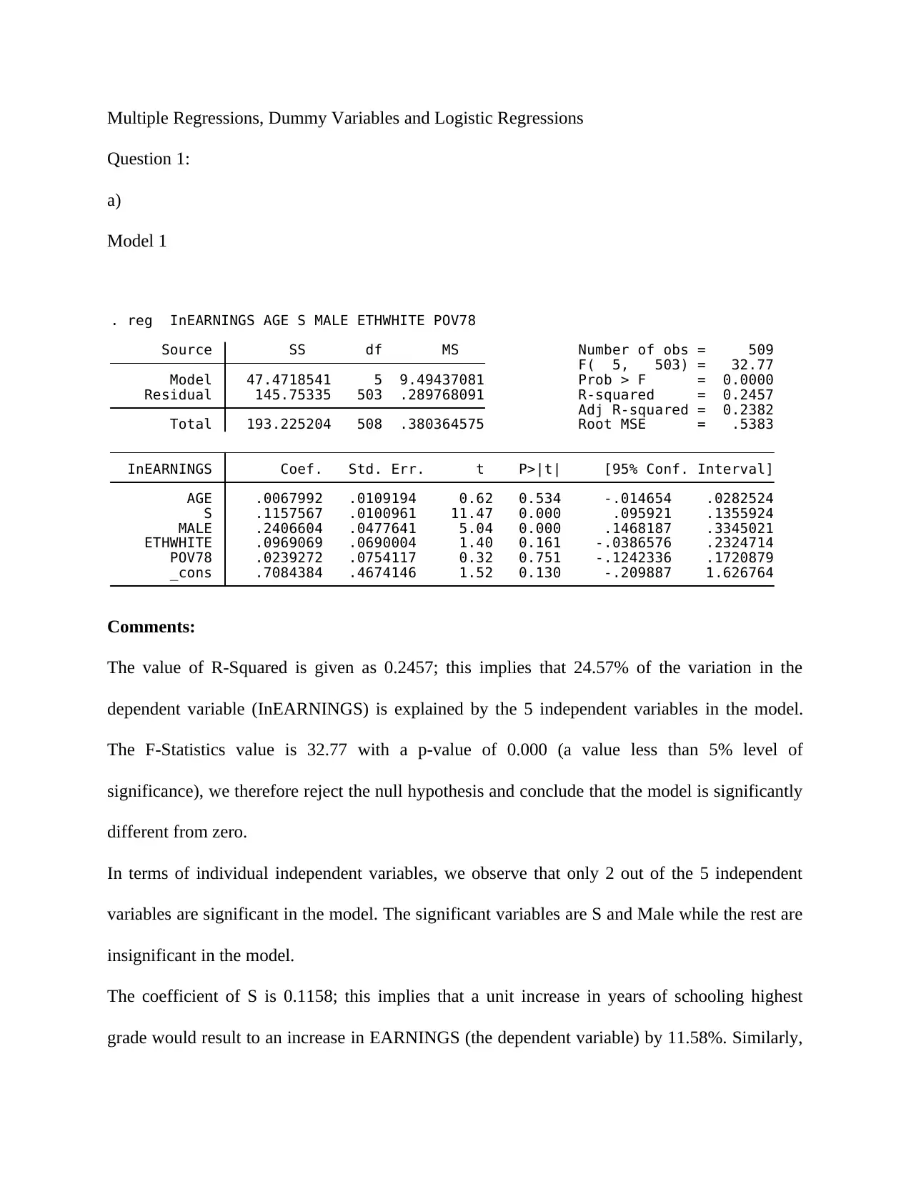
. reg InEARNINGS AGE S MALE ETHWHITE POV78
Comments:
The value of R-Squared is given as 0.2457; this implies that 24.57% of the variation in the
dependent variable (InEARNINGS) is explained by the 5 independent variables in the model.
The F-Statistics value is 32.77 with a p-value of 0.000 (a value less than 5% level of
significance), we therefore reject the null hypothesis and conclude that the model is significantly
different from zero.
In terms of individual independent variables, we observe that only 2 out of the 5 independent
variables are significant in the model. The significant variables are S and Male while the rest are
insignificant in the model.
The coefficient of S is 0.1158; this implies that a unit increase in years of schooling highest
grade would result to an increase in EARNINGS (the dependent variable) by 11.58%. Similarly,
Question 1:
a)
Model 1
_cons .7084384 .4674146 1.52 0.130 -.209887 1.626764
POV78 .0239272 .0754117 0.32 0.751 -.1242336 .1720879
ETHWHITE .0969069 .0690004 1.40 0.161 -.0386576 .2324714
MALE .2406604 .0477641 5.04 0.000 .1468187 .3345021
S .1157567 .0100961 11.47 0.000 .095921 .1355924
AGE .0067992 .0109194 0.62 0.534 -.014654 .0282524
InEARNINGS Coef. Std. Err. t P>|t| [95% Conf. Interval]
Total 193.225204 508 .380364575 Root MSE = .5383
Adj R-squared = 0.2382
Residual 145.75335 503 .289768091 R-squared = 0.2457
Model 47.4718541 5 9.49437081 Prob > F = 0.0000
F( 5, 503) = 32.77
Source SS df MS Number of obs = 509
. reg InEARNINGS AGE S MALE ETHWHITE POV78
Comments:
The value of R-Squared is given as 0.2457; this implies that 24.57% of the variation in the
dependent variable (InEARNINGS) is explained by the 5 independent variables in the model.
The F-Statistics value is 32.77 with a p-value of 0.000 (a value less than 5% level of
significance), we therefore reject the null hypothesis and conclude that the model is significantly
different from zero.
In terms of individual independent variables, we observe that only 2 out of the 5 independent
variables are significant in the model. The significant variables are S and Male while the rest are
insignificant in the model.
The coefficient of S is 0.1158; this implies that a unit increase in years of schooling highest
grade would result to an increase in EARNINGS (the dependent variable) by 11.58%. Similarly,
Paraphrase This Document
Need a fresh take? Get an instant paraphrase of this document with our AI Paraphraser
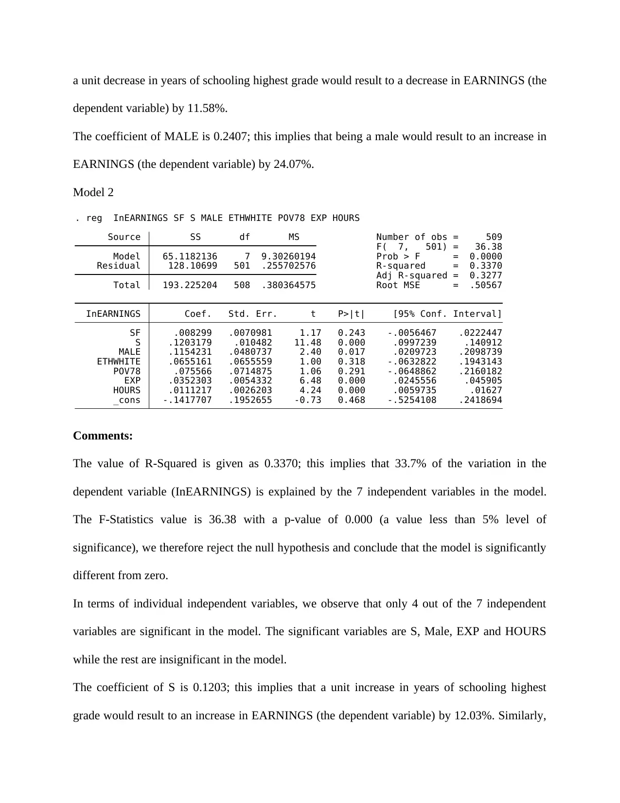
a unit decrease in years of schooling highest grade would result to a decrease in EARNINGS (the
dependent variable) by 11.58%.
The coefficient of MALE is 0.2407; this implies that being a male would result to an increase in
EARNINGS (the dependent variable) by 24.07%.
Model 2
_cons -.1417707 .1952655 -0.73 0.468 -.5254108 .2418694
HOURS .0111217 .0026203 4.24 0.000 .0059735 .01627
EXP .0352303 .0054332 6.48 0.000 .0245556 .045905
POV78 .075566 .0714875 1.06 0.291 -.0648862 .2160182
ETHWHITE .0655161 .0655559 1.00 0.318 -.0632822 .1943143
MALE .1154231 .0480737 2.40 0.017 .0209723 .2098739
S .1203179 .010482 11.48 0.000 .0997239 .140912
SF .008299 .0070981 1.17 0.243 -.0056467 .0222447
InEARNINGS Coef. Std. Err. t P>|t| [95% Conf. Interval]
Total 193.225204 508 .380364575 Root MSE = .50567
Adj R-squared = 0.3277
Residual 128.10699 501 .255702576 R-squared = 0.3370
Model 65.1182136 7 9.30260194 Prob > F = 0.0000
F( 7, 501) = 36.38
Source SS df MS Number of obs = 509
. reg InEARNINGS SF S MALE ETHWHITE POV78 EXP HOURS
Comments:
The value of R-Squared is given as 0.3370; this implies that 33.7% of the variation in the
dependent variable (InEARNINGS) is explained by the 7 independent variables in the model.
The F-Statistics value is 36.38 with a p-value of 0.000 (a value less than 5% level of
significance), we therefore reject the null hypothesis and conclude that the model is significantly
different from zero.
In terms of individual independent variables, we observe that only 4 out of the 7 independent
variables are significant in the model. The significant variables are S, Male, EXP and HOURS
while the rest are insignificant in the model.
The coefficient of S is 0.1203; this implies that a unit increase in years of schooling highest
grade would result to an increase in EARNINGS (the dependent variable) by 12.03%. Similarly,
a unit decrease in years of schooling highest grade would result to a decrease in EARNINGS (the
dependent variable) by 12.03%.
The coefficient of MALE is 0.1154; this implies that being a male would result to an increase in
EARNINGS (the dependent variable) by 11.54%.
The coefficient of EXP is 0.0352; this implies that a unit increase in total out-of school work
experience (years) would result to an increase in EARNINGS (the dependent variable) by 3.52%.
Similarly, a unit decrease in total out-of school work experience (years) would result to a
decrease in EARNINGS (the dependent variable) by 3.52%.
The coefficient of HOURS is 0.0111; this implies that a unit increase in usual number of hours
worked per week would result to an increase in EARNINGS (the dependent variable) by 1.11%.
Similarly, a unit decrease usual number of hours worked per week would result to a decrease in
EARNINGS (the dependent variable) by 1.11%.
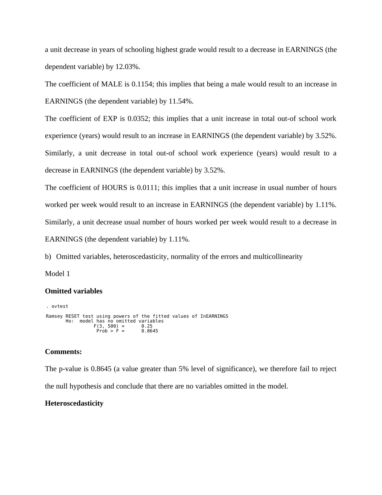
b) Omitted variables, heteroscedasticity, normality of the errors and multicollinearity
Model 1
Omitted variables
Prob > F = 0.8645
F(3, 500) = 0.25
Ho: model has no omitted variables
Ramsey RESET test using powers of the fitted values of InEARNINGS
. ovtest
Comments:
The p-value is 0.8645 (a value greater than 5% level of significance), we therefore fail to reject
the null hypothesis and conclude that there are no variables omitted in the model.
Heteroscedasticity
dependent variable) by 12.03%.
The coefficient of MALE is 0.1154; this implies that being a male would result to an increase in
EARNINGS (the dependent variable) by 11.54%.
The coefficient of EXP is 0.0352; this implies that a unit increase in total out-of school work
experience (years) would result to an increase in EARNINGS (the dependent variable) by 3.52%.
Similarly, a unit decrease in total out-of school work experience (years) would result to a
decrease in EARNINGS (the dependent variable) by 3.52%.
The coefficient of HOURS is 0.0111; this implies that a unit increase in usual number of hours
worked per week would result to an increase in EARNINGS (the dependent variable) by 1.11%.
Similarly, a unit decrease usual number of hours worked per week would result to a decrease in
EARNINGS (the dependent variable) by 1.11%.
b) Omitted variables, heteroscedasticity, normality of the errors and multicollinearity
Model 1
Omitted variables
Prob > F = 0.8645
F(3, 500) = 0.25
Ho: model has no omitted variables
Ramsey RESET test using powers of the fitted values of InEARNINGS
. ovtest
Comments:
The p-value is 0.8645 (a value greater than 5% level of significance), we therefore fail to reject
the null hypothesis and conclude that there are no variables omitted in the model.
Heteroscedasticity
⊘ This is a preview!⊘
Do you want full access?
Subscribe today to unlock all pages.
Trusted by 1+ million students worldwide
Total 19.93 23 0.6461
Kurtosis 4.78 1 0.0288
Skewness 5.14 5 0.3985
Heteroskedasticity 10.01 17 0.9034
Source chi2 df p
Cameron & Trivedi's decomposition of IM-test
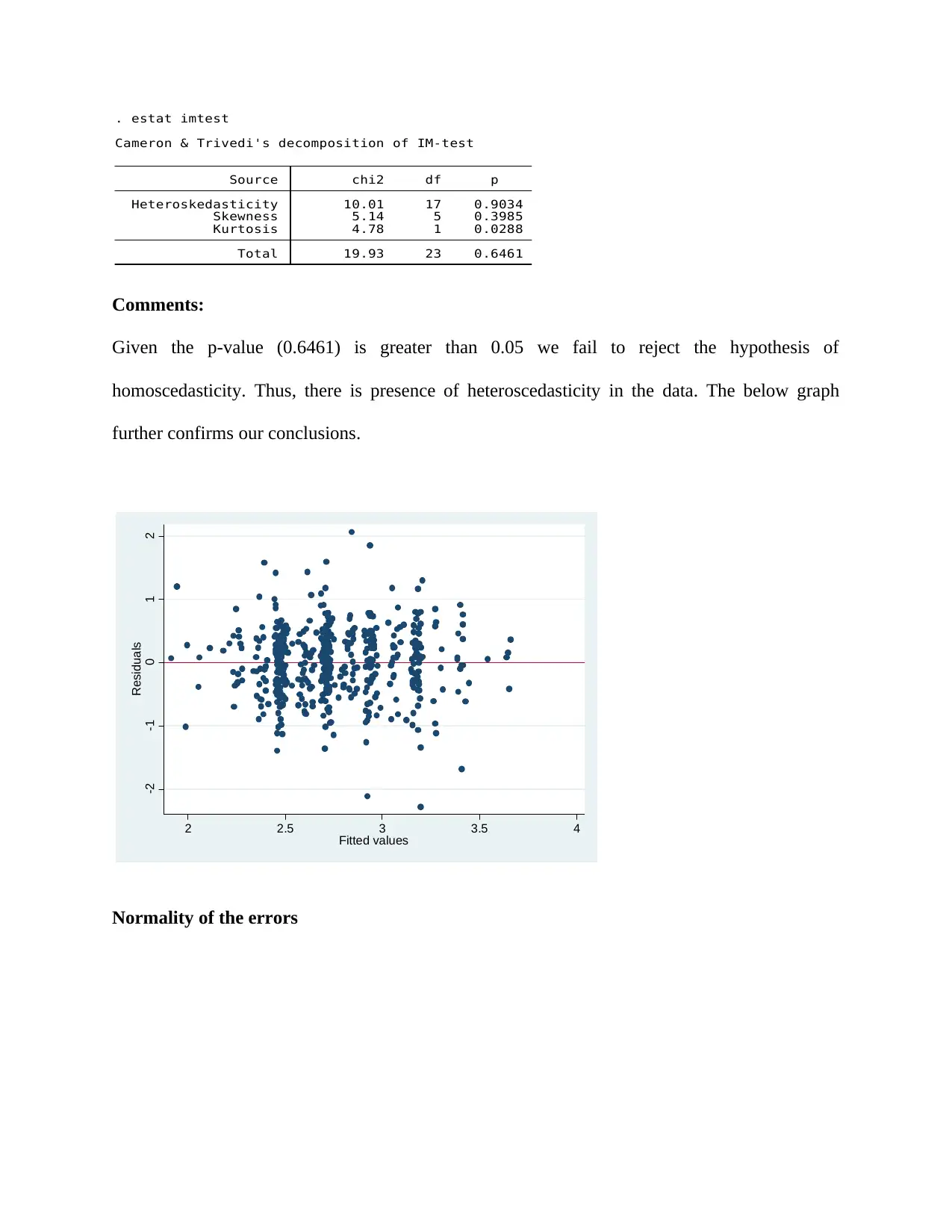
. estat imtest
Comments:
Given the p-value (0.6461) is greater than 0.05 we fail to reject the hypothesis of
homoscedasticity. Thus, there is presence of heteroscedasticity in the data. The below graph
further confirms our conclusions.
-2 -1 0 1 2
Residuals
2 2.5 3 3.5 4
Fitted values
Normality of the errors
Kurtosis 4.78 1 0.0288
Skewness 5.14 5 0.3985
Heteroskedasticity 10.01 17 0.9034
Source chi2 df p
Cameron & Trivedi's decomposition of IM-test
. estat imtest
Comments:
Given the p-value (0.6461) is greater than 0.05 we fail to reject the hypothesis of
homoscedasticity. Thus, there is presence of heteroscedasticity in the data. The below graph
further confirms our conclusions.
-2 -1 0 1 2
Residuals
2 2.5 3 3.5 4
Fitted values
Normality of the errors
Paraphrase This Document
Need a fresh take? Get an instant paraphrase of this document with our AI Paraphraser
0 .2 .4 .6 .8
Density
-2 -1 0 1 2
Residuals
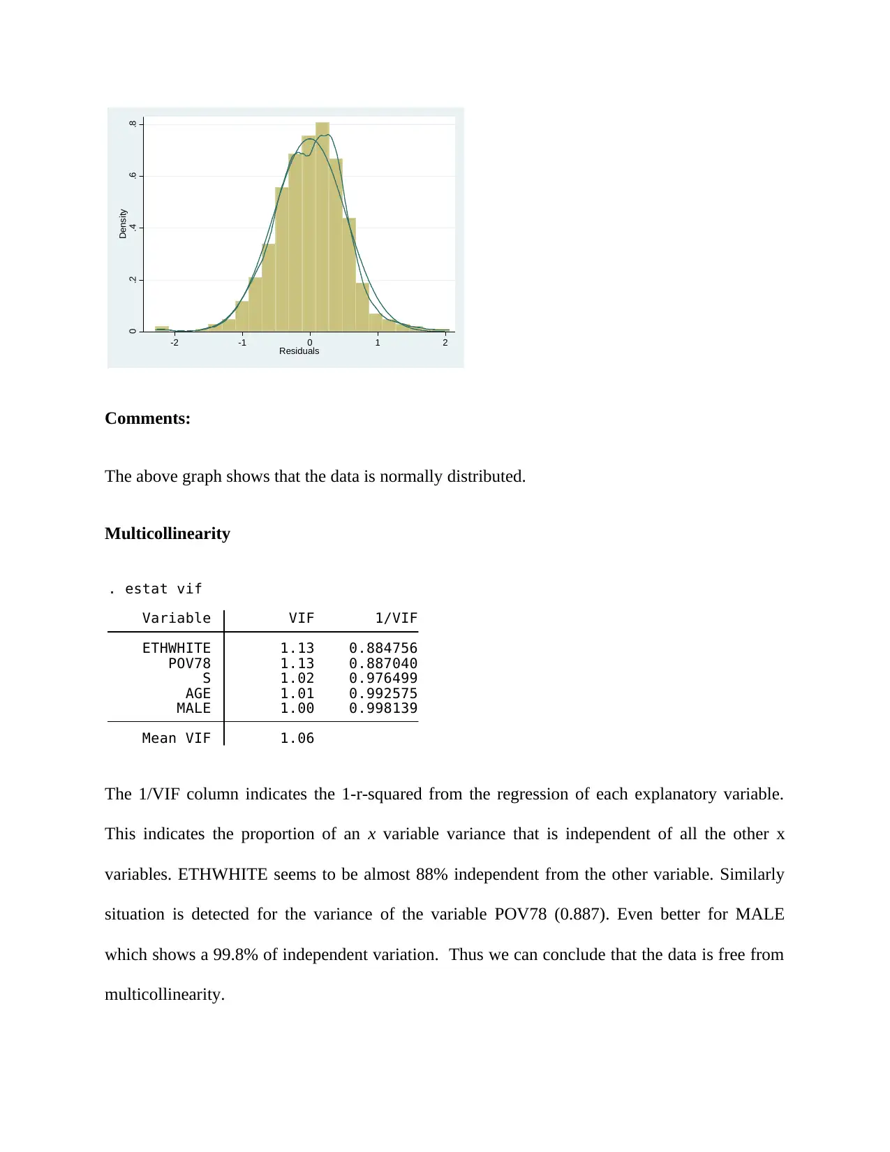
Comments:
The above graph shows that the data is normally distributed.
Multicollinearity
Mean VIF 1.06
MALE 1.00 0.998139
AGE 1.01 0.992575
S 1.02 0.976499
POV78 1.13 0.887040
ETHWHITE 1.13 0.884756
Variable VIF 1/VIF
. estat vif
The 1/VIF column indicates the 1-r-squared from the regression of each explanatory variable.
This indicates the proportion of an x variable variance that is independent of all the other x
variables. ETHWHITE seems to be almost 88% independent from the other variable. Similarly
situation is detected for the variance of the variable POV78 (0.887). Even better for MALE
which shows a 99.8% of independent variation. Thus we can conclude that the data is free from
multicollinearity.
Density
-2 -1 0 1 2
Residuals
Comments:
The above graph shows that the data is normally distributed.
Multicollinearity
Mean VIF 1.06
MALE 1.00 0.998139
AGE 1.01 0.992575
S 1.02 0.976499
POV78 1.13 0.887040
ETHWHITE 1.13 0.884756
Variable VIF 1/VIF
. estat vif
The 1/VIF column indicates the 1-r-squared from the regression of each explanatory variable.
This indicates the proportion of an x variable variance that is independent of all the other x
variables. ETHWHITE seems to be almost 88% independent from the other variable. Similarly
situation is detected for the variance of the variable POV78 (0.887). Even better for MALE
which shows a 99.8% of independent variation. Thus we can conclude that the data is free from
multicollinearity.
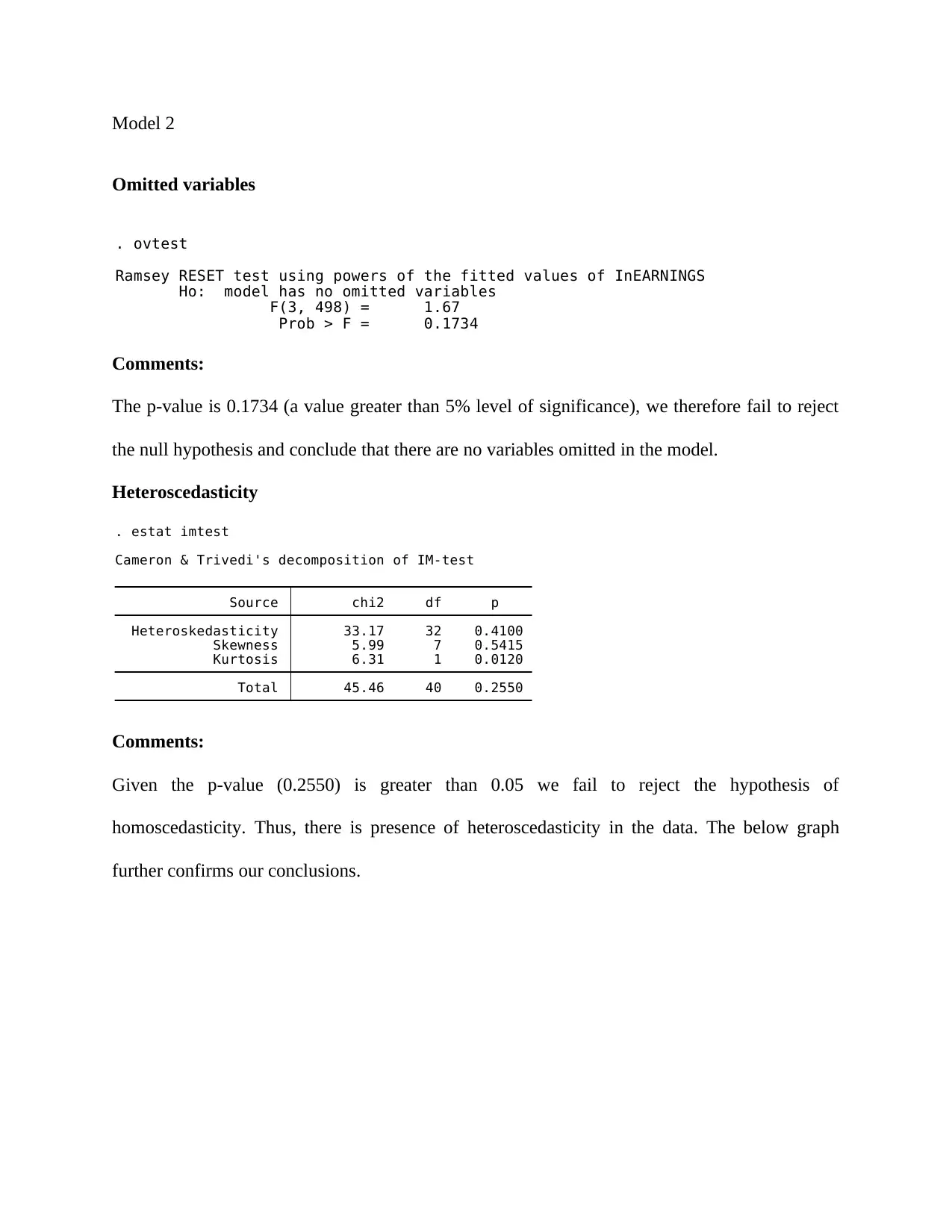
Model 2
Omitted variables
Prob > F = 0.1734
F(3, 498) = 1.67
Ho: model has no omitted variables
Ramsey RESET test using powers of the fitted values of InEARNINGS
. ovtest
Comments:
The p-value is 0.1734 (a value greater than 5% level of significance), we therefore fail to reject
the null hypothesis and conclude that there are no variables omitted in the model.
Heteroscedasticity
Total 45.46 40 0.2550
Kurtosis 6.31 1 0.0120
Skewness 5.99 7 0.5415
Heteroskedasticity 33.17 32 0.4100
Source chi2 df p
Cameron & Trivedi's decomposition of IM-test
. estat imtest
Comments:
Given the p-value (0.2550) is greater than 0.05 we fail to reject the hypothesis of
homoscedasticity. Thus, there is presence of heteroscedasticity in the data. The below graph
further confirms our conclusions.
⊘ This is a preview!⊘
Do you want full access?
Subscribe today to unlock all pages.
Trusted by 1+ million students worldwide
1 out of 23
Your All-in-One AI-Powered Toolkit for Academic Success.
+13062052269
info@desklib.com
Available 24*7 on WhatsApp / Email
![[object Object]](/_next/static/media/star-bottom.7253800d.svg)
Unlock your academic potential
Copyright © 2020–2026 A2Z Services. All Rights Reserved. Developed and managed by ZUCOL.