Higher Education: Computer-Aided Analysis of Non-Linear Equations
VerifiedAdded on 2022/08/13
|10
|1589
|14
Homework Assignment
AI Summary
This assignment solution delves into the analysis of non-linear equations, covering various methods for their resolution, including substitution, quadratic formula, elimination, and factorization. It elucidates the enhanced accuracy of Newton-Raphson's second method compared to the first, alongside methods for solving large systems of simultaneous equations using linear algebra packages. The solution also addresses the error-prone nature of Cramer's method, the stages of Gaussian elimination, and techniques to minimize round-off errors. Furthermore, it explores matrix pivoting, the coefficient of multiple determination, data types used in curve fitting, eigenproblem solutions, interpolation methods, numerical integration, and the Gauss quadrature principle. The assignment draws on cited references to support the explanations.

1
COMPUTER AIDED ANALYSIS
By Name
Course
Instructor
Institution
Location
Date
COMPUTER AIDED ANALYSIS
By Name
Course
Instructor
Institution
Location
Date
Paraphrase This Document
Need a fresh take? Get an instant paraphrase of this document with our AI Paraphraser
2
1. Methods used for solve non-linear equations.
Nonlinear equations are a classification of two or more equations with two or more variables
containing at least one equation that is not linear. Methods used to solve them include;
Substitution method
Quadratic formula
Elimination method
Factorization (Petkovic, et al., 2013, p. 76)
2. Why Newton-Rap son’s second method is more accurate than non-linear equations.
It does so using quadratic method when the method converges-Quadratic equation
is an equation of the subsequent degree. That means it has at least one term which
is squared. This eases and simplifies the equations.
The method is very simple to apply i.e. the method is very simple and easy to
articulate and solve as its basis is on the second degree level. (Fletcher, 2016, p.
233)
Has great local convergence. It is based on finding a root of a function and
comprises at the minimum of one term which is squared. This eases and simplifies
the equations.
3. Method used to solve a large number of simultaneous equations.
Linear equations system
The Linear algebra packages are used to calculate large number of simultaneous
equation. Linear equation has rational polynomial names
Kappa. Linear Solve command and option to find out unknown vector x in MAPLE 18.
(Fletcher, 2011, p. 347)
3
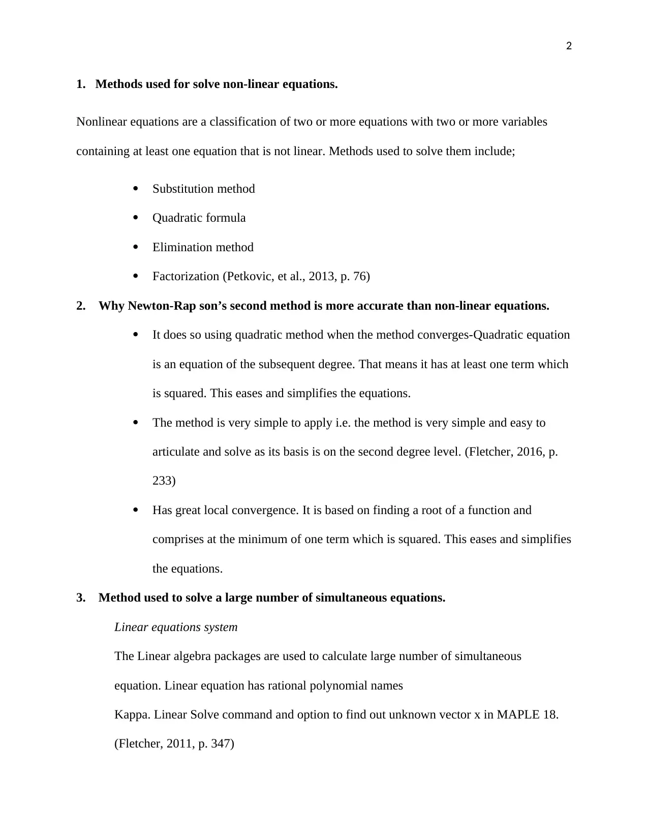
Figure 1: Showing a sample of Linear Equations solution.
4. When considering using Cramer’s method to solve the problem [𝐴][𝑥] = {𝑏}, in what
situation would using Cramer’s method be considered error prone?
When considering using Cramer’s method, the method is considered error prone during the
evaluation of determinants (Kelley, 2016, p. 665).
5. The first phase of Gaussian elimination
The stages involved in Gaussian elimination include:
i. Examine the first column of matrix [A/b] beginning at the right top to the bottom for the
first and non-zero on your left bottom., and in case there is need, the next column (usually
in a scenario which has all its coefficients agreeing to the first variable are zero, the third
column and the series continuous. The entry obtained is referred to as the current pivot.
ii. If there is need, interchanging the row that has the current pivot with the first row can be
done.
⊘ This is a preview!⊘
Do you want full access?
Subscribe today to unlock all pages.
Trusted by 1+ million students worldwide
4
iii. Does not touch the first row i.e. the row enclosing the pivot, then subtract suitable
multiples of the first row from all the remaining rows so that to attain all zeros which are
under the existing pivot column.
iv. Carry out the previous stages on the sub matrix containing all the elements that are under
and to the right of the existing pivot.
v. End the moment there is no new pivot that can be obtained (Saaty, 2012, p. 265).
6. How round-off errors can be minimized during Gaussian elimination
The round-off errors can be avoided through the careful selection of the ap,i = maxikn|ak,i| and
swap row p with row i. This ensures that all the pivots we use are large as possible to reduce the
possible round-off errors.
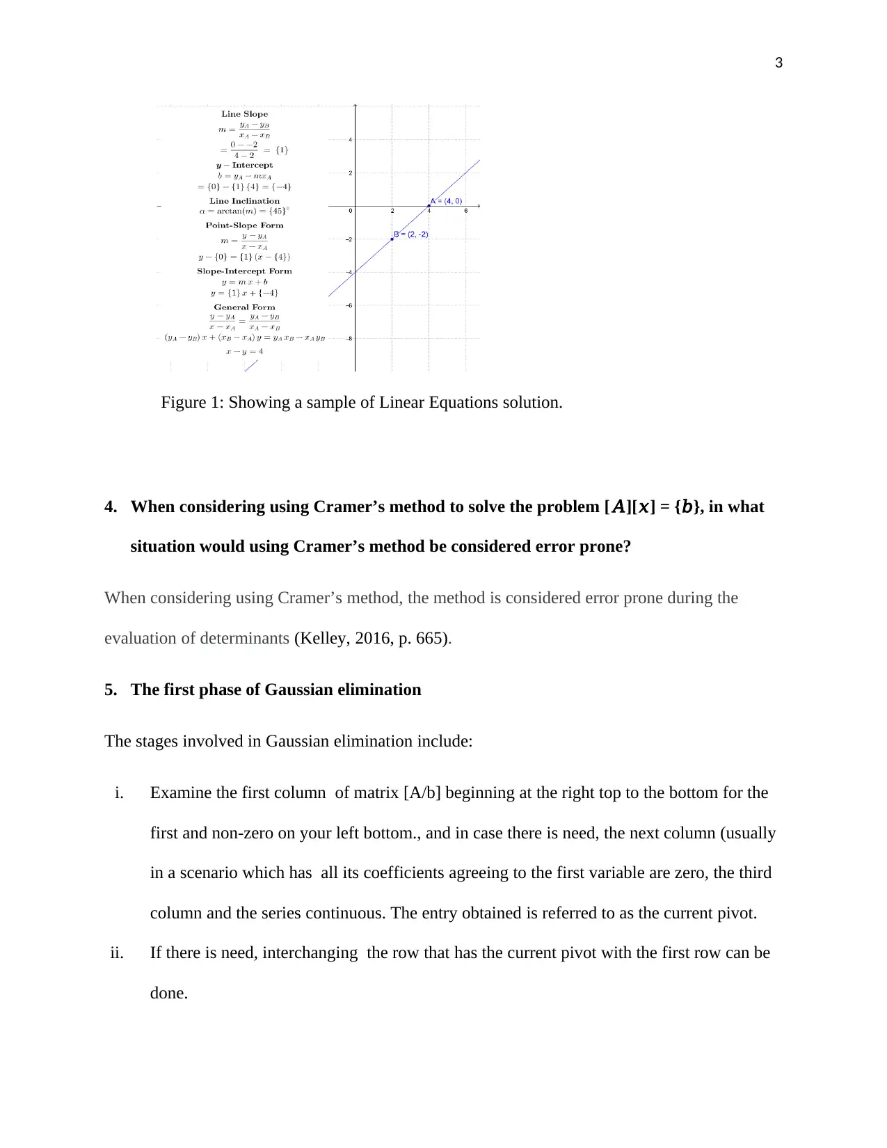
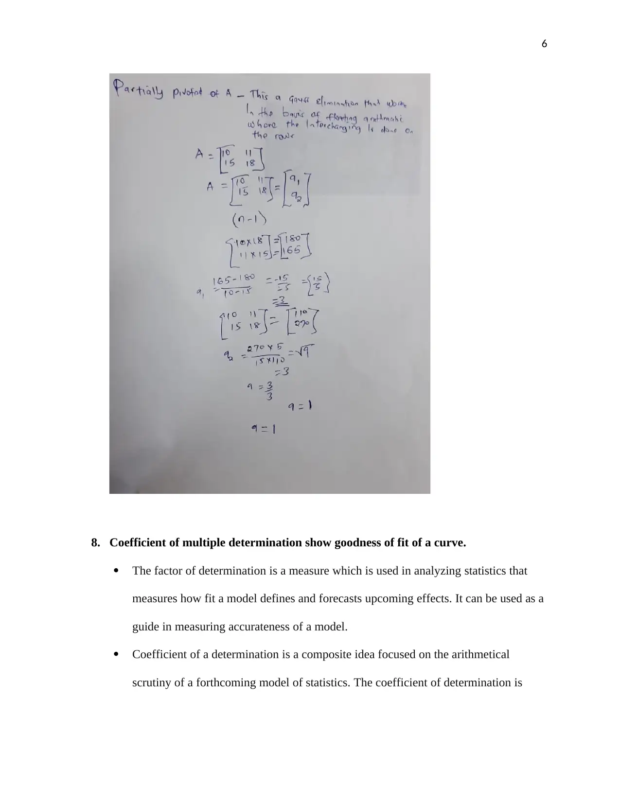
7. While considering this matrix; Find the partially pivoted matrix of A.
The main aim of pivoting a matrix is to create the element that is directly above or under the top
one into a zero. The pivotal element is that element which is on the left hand side of a given
matrix that you want the elements that are above and below to be zero. Usually, the element is
one.
A row can be multiplied by a constant number which is not a zero and adding it to a non-zero
multiple of an alternative row, replacing the row.
Therefore, in case the requirement is to pivot on a one number, then the second elementary row
operation should be used. It is divided by a row on the upper element to create it into one.
Division leads into fractions. If the fractions are not used in this case, the mistakes are likely to
be made.
Pivoting process
iii. Does not touch the first row i.e. the row enclosing the pivot, then subtract suitable
multiples of the first row from all the remaining rows so that to attain all zeros which are
under the existing pivot column.
iv. Carry out the previous stages on the sub matrix containing all the elements that are under
and to the right of the existing pivot.
v. End the moment there is no new pivot that can be obtained (Saaty, 2012, p. 265).
6. How round-off errors can be minimized during Gaussian elimination
The round-off errors can be avoided through the careful selection of the ap,i = maxikn|ak,i| and
swap row p with row i. This ensures that all the pivots we use are large as possible to reduce the
possible round-off errors.
7. While considering this matrix; Find the partially pivoted matrix of A.
The main aim of pivoting a matrix is to create the element that is directly above or under the top
one into a zero. The pivotal element is that element which is on the left hand side of a given
matrix that you want the elements that are above and below to be zero. Usually, the element is
one.
A row can be multiplied by a constant number which is not a zero and adding it to a non-zero
multiple of an alternative row, replacing the row.
Therefore, in case the requirement is to pivot on a one number, then the second elementary row
operation should be used. It is divided by a row on the upper element to create it into one.
Division leads into fractions. If the fractions are not used in this case, the mistakes are likely to
be made.
Pivoting process
Paraphrase This Document
Need a fresh take? Get an instant paraphrase of this document with our AI Paraphraser
5
The process of pivoting works well since a common multiple of two figures is found by
multiplying two numbers together. It is highly recommended to pivot on one. That means you
are multiplying by one. It is also recommended that the main diagonal be pivoted. You can start
from the upper left and do it your way down to the lower right. Once every row and column is
pivoted, the cleared column should stay like that. The area of pivoting is made to clear the
column of the pivot. Therefore, if you pick a column which has zero(s) in it saves time since
there is no need to change the row which has the zero.
How to select a pivot
Choose the column which has many zeros
Utilize that row or column only once
If possible, pivot on a one number
Pivoting should be done on the leading diagonal;
Don’t pivot a zero number
Don’t pivot the right side of the hand.
6
8. Coefficient of multiple determination show goodness of fit of a curve.
The factor of determination is a measure which is used in analyzing statistics that
measures how fit a model defines and forecasts upcoming effects. It can be used as a
guide in measuring accurateness of a model.
Coefficient of a determination is a composite idea focused on the arithmetical
scrutiny of a forthcoming model of statistics. The coefficient of determination is
⊘ This is a preview!⊘
Do you want full access?
Subscribe today to unlock all pages.
Trusted by 1+ million students worldwide
7
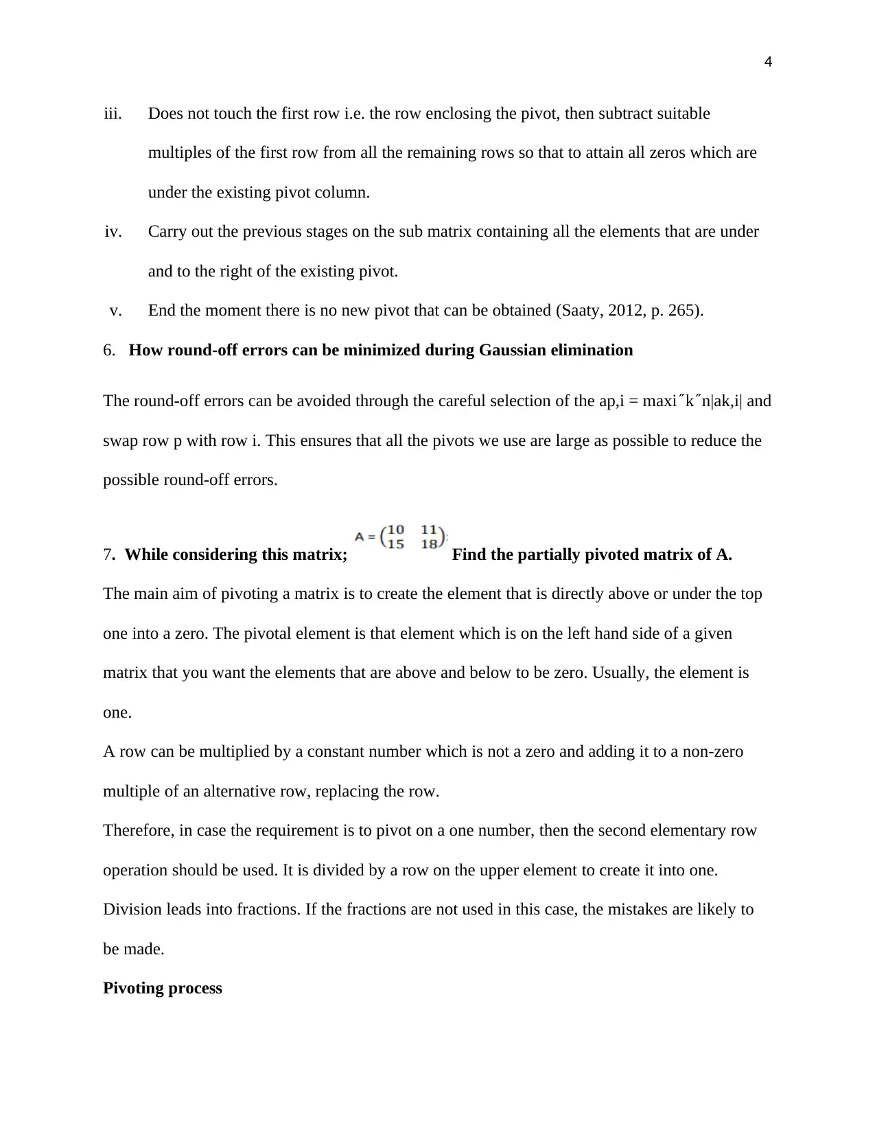
used to explain how much variability of one factor can be can be caused by its
relationship to another factor.
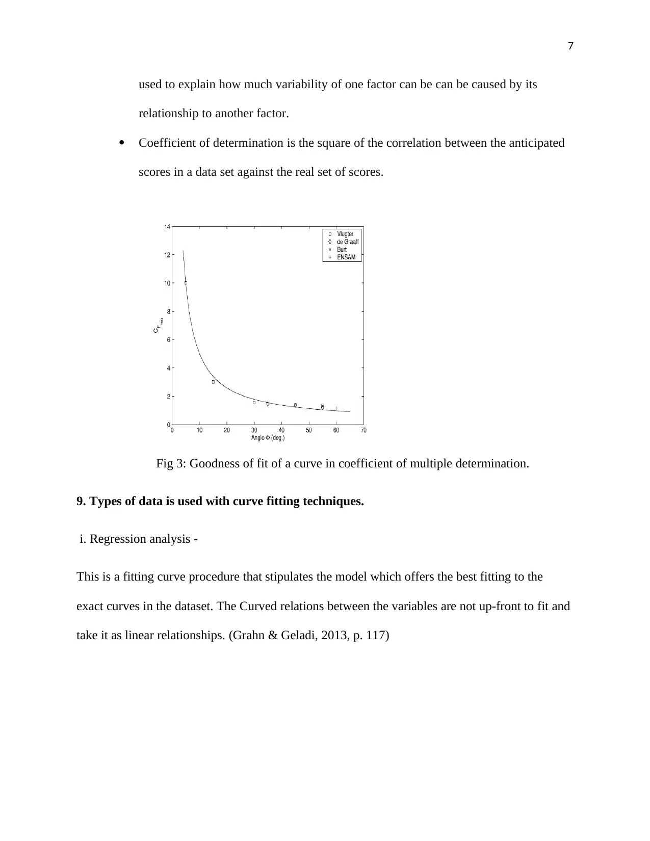
Coefficient of determination is the square of the correlation between the anticipated
scores in a data set against the real set of scores.
Fig 3: Goodness of fit of a curve in coefficient of multiple determination.
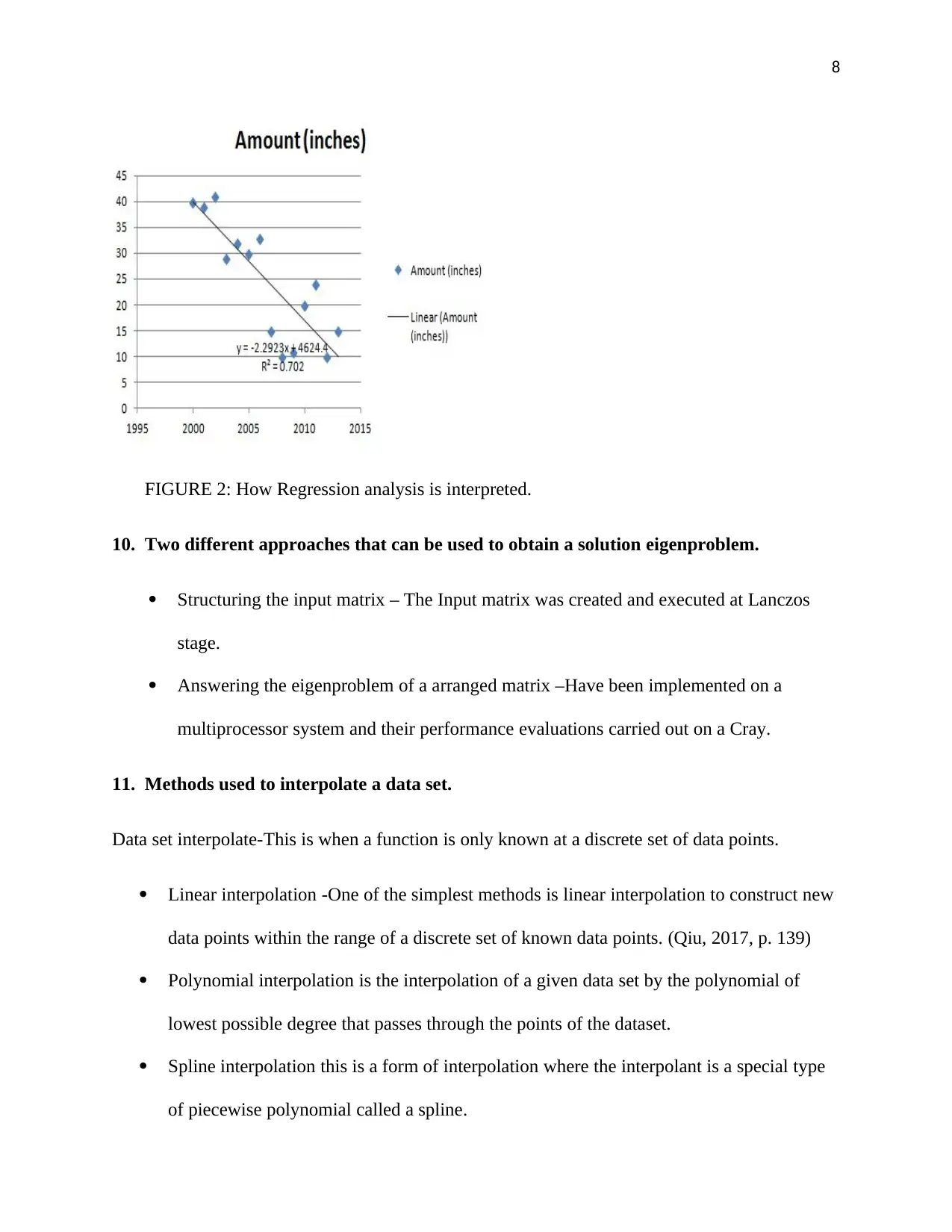
9. Types of data is used with curve fitting techniques.
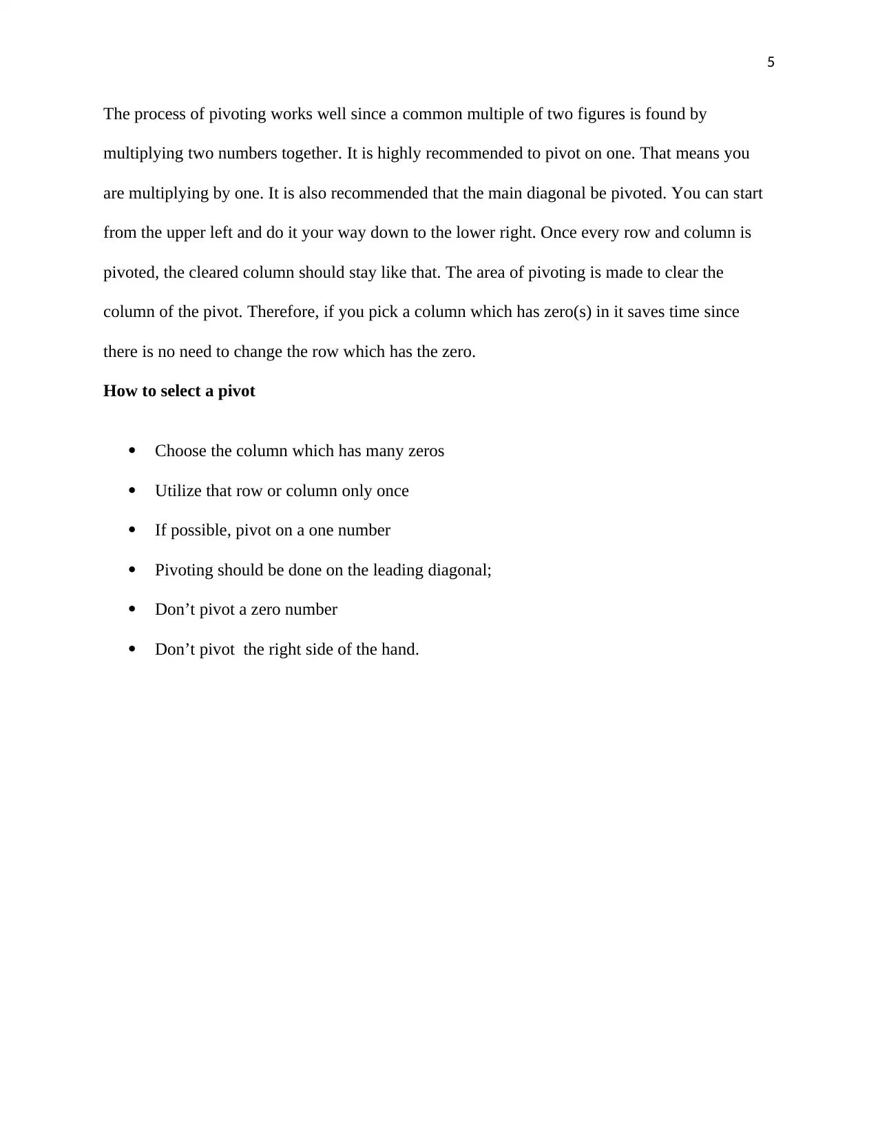
i. Regression analysis -
This is a fitting curve procedure that stipulates the model which offers the best fitting to the
exact curves in the dataset. The Curved relations between the variables are not up-front to fit and
take it as linear relationships. (Grahn & Geladi, 2013, p. 117)
used to explain how much variability of one factor can be can be caused by its
relationship to another factor.
Coefficient of determination is the square of the correlation between the anticipated
scores in a data set against the real set of scores.
Fig 3: Goodness of fit of a curve in coefficient of multiple determination.
9. Types of data is used with curve fitting techniques.
i. Regression analysis -
This is a fitting curve procedure that stipulates the model which offers the best fitting to the
exact curves in the dataset. The Curved relations between the variables are not up-front to fit and
take it as linear relationships. (Grahn & Geladi, 2013, p. 117)
Paraphrase This Document
Need a fresh take? Get an instant paraphrase of this document with our AI Paraphraser
8
FIGURE 2: How Regression analysis is interpreted.
10. Two different approaches that can be used to obtain a solution eigenproblem.
Structuring the input matrix – The Input matrix was created and executed at Lanczos
stage.
Answering the eigenproblem of a arranged matrix –Have been implemented on a
multiprocessor system and their performance evaluations carried out on a Cray.
11. Methods used to interpolate a data set.
Data set interpolate-This is when a function is only known at a discrete set of data points.
Linear interpolation -One of the simplest methods is linear interpolation to construct new
data points within the range of a discrete set of known data points. (Qiu, 2017, p. 139)
Polynomial interpolation is the interpolation of a given data set by the polynomial of
lowest possible degree that passes through the points of the dataset.
Spline interpolation this is a form of interpolation where the interpolant is a special type
of piecewise polynomial called a spline.
9
12. Common method of numerical integration
The most common method used in numerical integration is Newton-cotes Integration Formula. It
solves integrals in two situations which include replacing the complicated integrand function, or
tabulated data by an approximating function easy to integrate like a polynomial.
13. Describe the basic principle of the Gauss quadrature.
The basic principle of Gauss quadrature states that the optimal abscissas of the m-point gussian
quadrature formulas are precisely the roots of the orthogonal polynomial for the same interval
and weighing function.
References
Fletcher, R., 2011. Practical Methods of Optimization. 3rd ed. Texas: John Wiley & Sons.
⊘ This is a preview!⊘
Do you want full access?
Subscribe today to unlock all pages.
Trusted by 1+ million students worldwide
10
Fletcher, R., 2016. Practical Methods of Optimization. 2nd ed. New York: John Wiley & Sons.
Grahn, H. & Geladi, P., 2013. Techniques and Applications of Hyperspectral Image Analysis.
2nd ed. Paris: s.n.
Kelley, C., 2016. Solving Nonlinear Equations with Newton's Method. 3rd ed. Chicago: SIAM,.
Optimization, P. M. o., 2014. R. Fletcher. 4th ed. New York: John Wiley & Sons.
Petkovic, M., Neta, B., Petkovic, L. & Dzunic, J., 2013. Multipoint Methods for Solving
Nonlinear Equations. 4th ed. London: Academic Press.
Qiu, P., 2017. Image Processing and Jump Regression Analysis. 4th ed. Paris: John Wiley &
Sons.
Saaty, T., 2012. Modern Nonlinear Equations. 5th ed. sydney: Courier Corporation.
1 out of 10
Your All-in-One AI-Powered Toolkit for Academic Success.
+13062052269
info@desklib.com
Available 24*7 on WhatsApp / Email
![[object Object]](/_next/static/media/star-bottom.7253800d.svg)
Unlock your academic potential
Copyright © 2020–2026 A2Z Services. All Rights Reserved. Developed and managed by ZUCOL.