Exploring Nonlinear Approximation Techniques and Their Applications

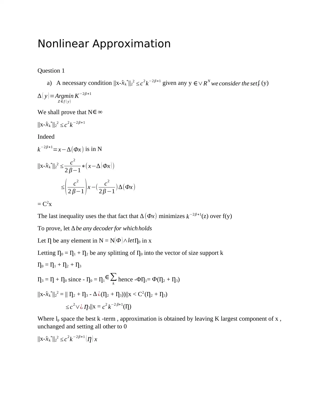
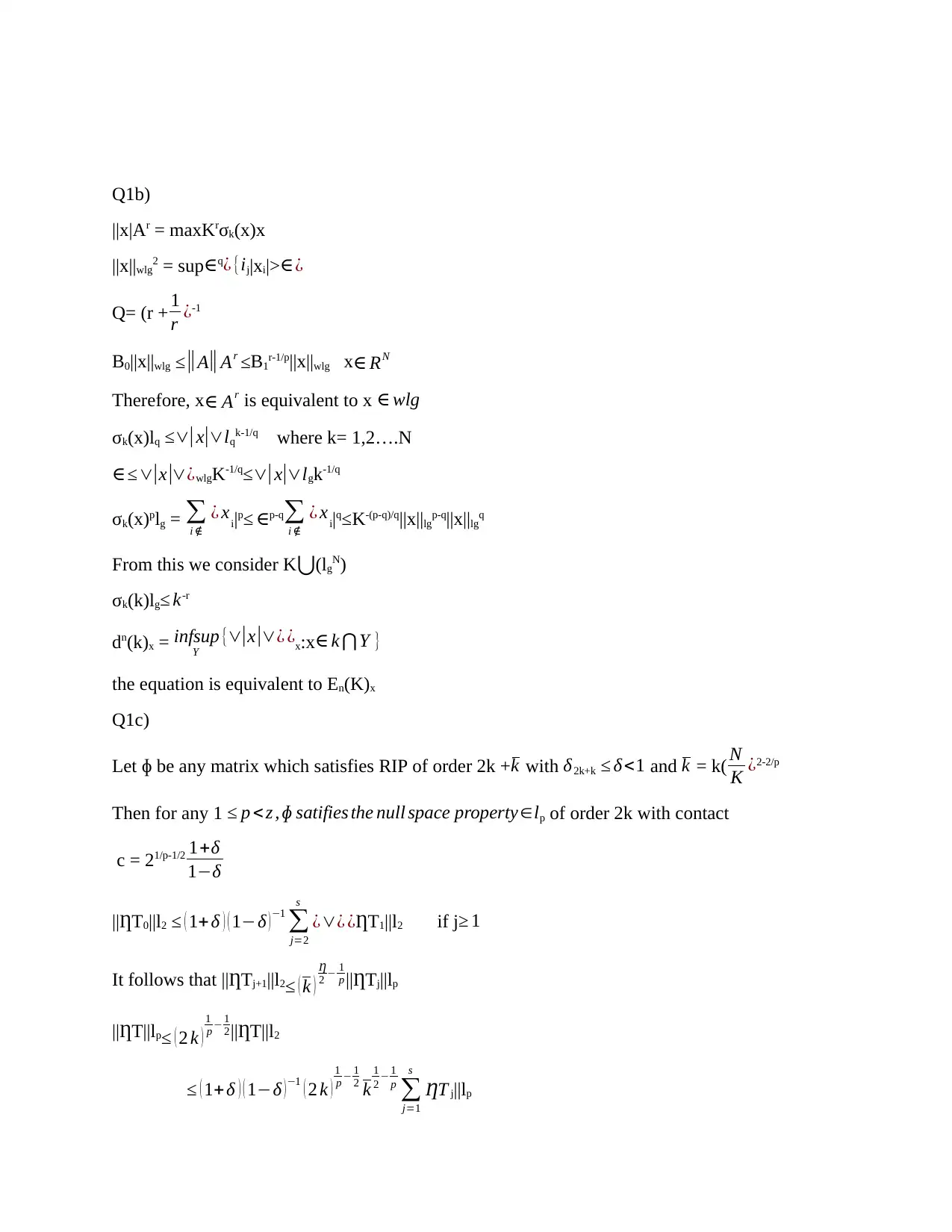
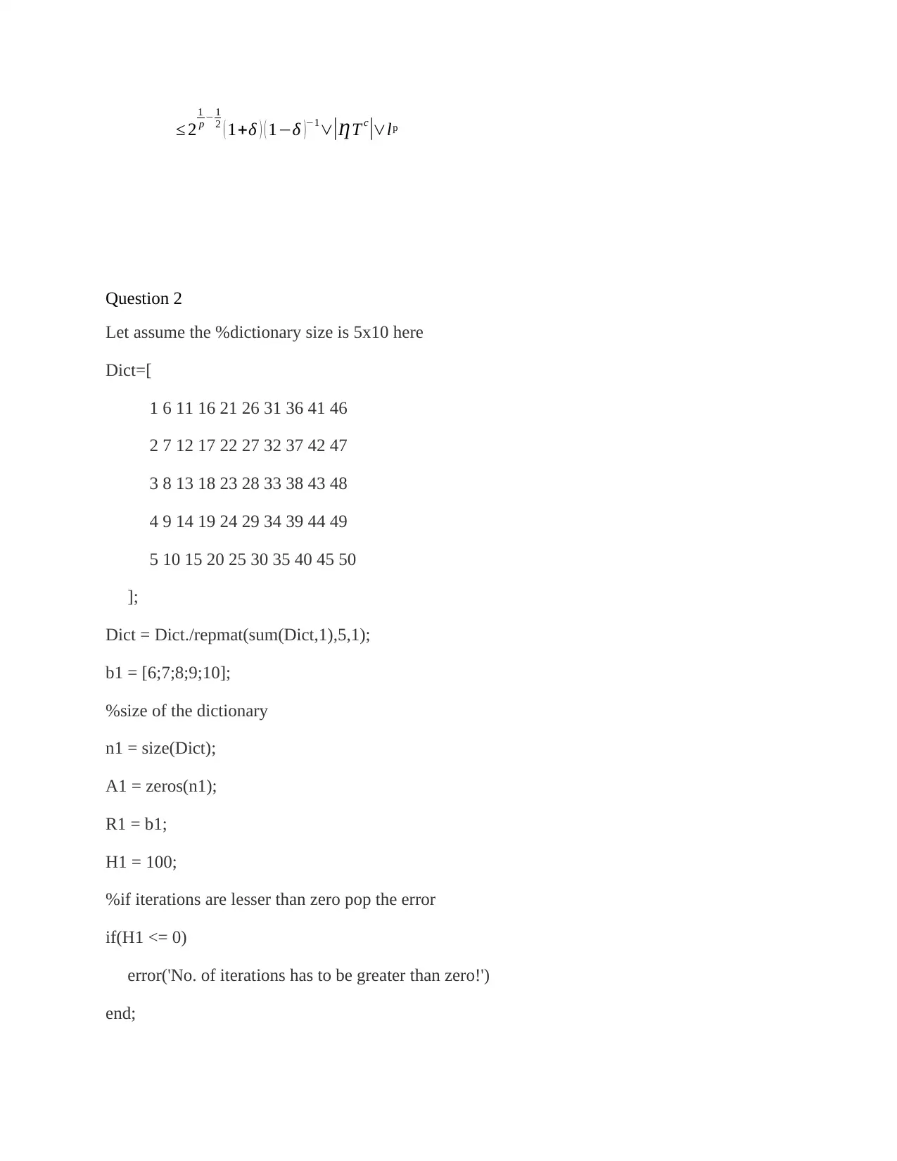
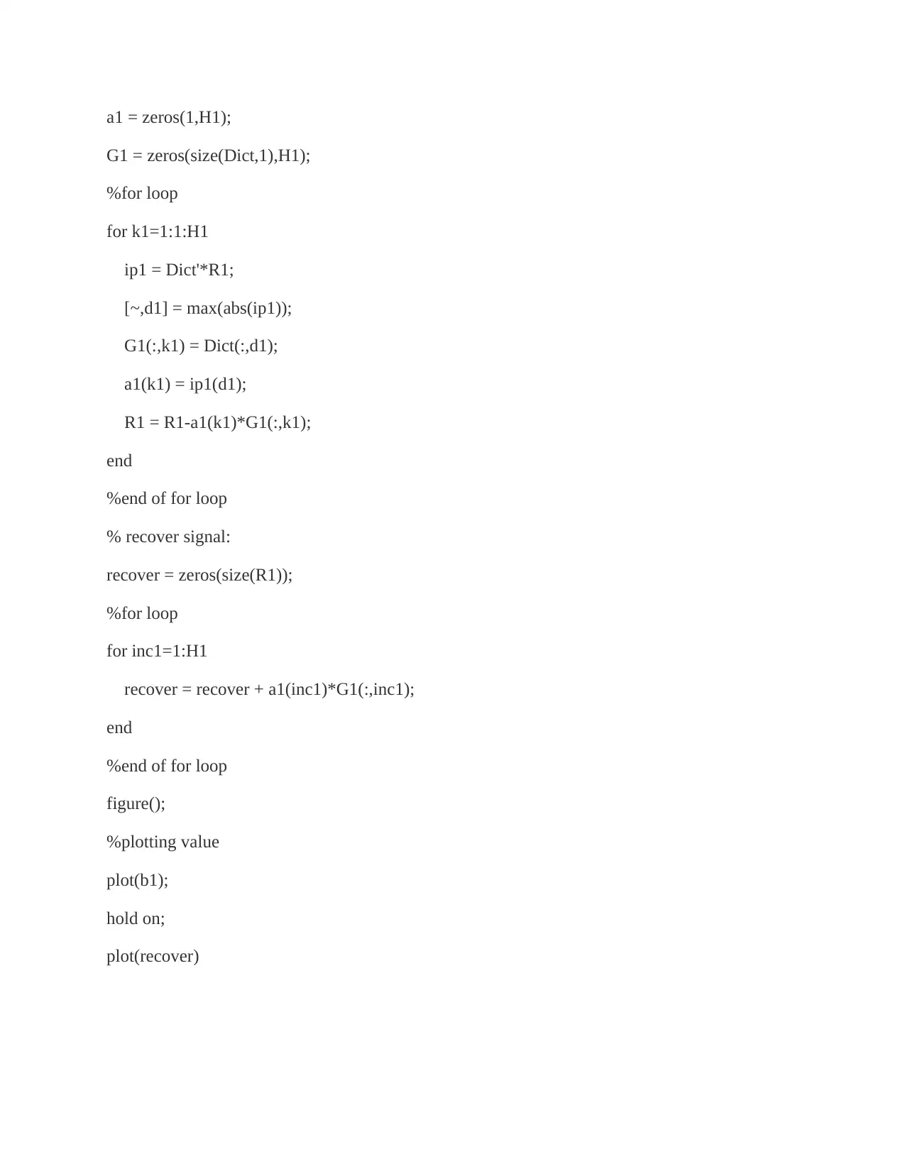
This academic exercise tackles the fundamentals of nonlinear approximation with an emphasis on achieving sparse representations in signal processing. The assignment is structured around three main questions: proving necessary conditions using Restricted Isometry Property (RIP), exploring dictionary learning via Matching Pursuit, and calculating eigenvalues for matrix approximations. MATLAB code snippets are provided to illustrate practical implementations of these theoretical concepts, culminating in applications such as least squares solutions for Fourier coefficients.

Nonlinear Approximation
Question 1
a) A necessary condition ||x- ^xk*||22 ≤ c2 k−2 β +1 given any y ∈∨RN we consider the setʄ (y)
∆ ( y ) =Argmin
Z ∈ f ( y)
K−2 β +1
We shall prove that N∈ ∞
||x- ^xk*||22 ≤ c2 k−2 β +1
Indeed
k−2 β +1=x−∆(Φx ) is in N
||x- ^xk*||22 ≤ c2
2 β−1∗(x−∆ ( Φx ) )
≤ ( c2
2 β−1 )x −( c2
2 β −1 ) ∆(Φx )
= C2x
The last inequality uses the that fact that ∆ (Φx) minimizes k−2 β +1(z) over f(y)
To prove, let ∆ be any decoder for which holds
Let Ƞ be any element in N = N ( Φ )∧letȠ0 in x
Letting Ƞ0 = Ƞ1 + Ƞ2 be any splitting of Ƞ0 into the vector of size support k
Ƞ0 = Ƞ1 + Ƞ2 + Ƞ3
Ƞ3 = Ƞ + Ƞ0 since - Ƞ0 = Ƞ1∈∑
k hence -ΦȠ1= Φ(Ƞ2 + Ƞ3)
||x- ^xk*||22 = || Ƞ2 + Ƞ3 - ∆ ¿(Ƞ2 + Ƞ3))||x < C2 (Ƞ2 + Ƞ3)
≤ c2∨¿ Ƞ3||x = c2 k−2 β+1(Ƞ)
Where lp space the best k -term , approximation is obtained by leaving K largest component of x ,
unchanged and setting all other to 0
||x- ^xk*||22 ≤ c2 k−2 β +1 ( Ƞ ) x

Q1b)
||x|Ar = maxKrσk(x)x
||x||wlg2 = sup∈q
¿ {ij|xi|>∈¿
Q= (r + 1
r ¿-1
B0||x||wlg ≤ ||A|| Ar ≤B1r-1/p||x||wlg x∈ RN
Therefore, x∈ Ar is equivalent to x ∈ wlg
σk(x)lq ≤∨|x|∨lqk-1/q where k= 1,2….N
∈≤∨|x|∨¿wlgK-1/q
≤∨| x|∨lgk-1/q
σk(x)plg = ∑
i ∉
¿ xi|p≤ ∈p-q∑
i ∉
¿ xi|q≤K-(p-q)/q||x||lgp-q||x||lgq
From this we consider K⋃(lgN)
σk(k)lg≤ k-r
dn(k)x = infsup
Y
{∨|x|∨¿ ¿x:x∈ k ⋂ Y }
the equation is equivalent to En(K)x
Q1c)
Let ɸ be any matrix which satisfies RIP of order 2k +k with δ2k+k ≤ δ<1 and k = k( N
K ¿2-2/p
Then for any 1 ≤ p < z , ɸ satifies the null space property∈lp of order 2k with contact
c = 21/p-1/2 1+δ
1−δ
||ȠT0||l2 ≤ ( 1+ δ ) ( 1−δ )−1
∑
j=2
s
¿∨¿ ¿ȠT1||l2 if j≥ 1
It follows that ||ȠTj+1||l2≤ ( k )
Ƞ
2 − 1
p ||ȠTj||lp
||ȠT||lp≤ ( 2 k )
1
p − 1
2||ȠT||l2
≤ ( 1+δ ) ( 1−δ )−1 ( 2 k )
1
p − 1
2 k
1
2 − 1
p ∑
j=1
s
ȠT j||lp

≤ 2
1
p − 1
2 ( 1+δ ) ( 1−δ )−1∨|ȠT c
|∨lp
Question 2
Let assume the %dictionary size is 5x10 here
Dict=[
1 6 11 16 21 26 31 36 41 46
2 7 12 17 22 27 32 37 42 47
3 8 13 18 23 28 33 38 43 48
4 9 14 19 24 29 34 39 44 49
5 10 15 20 25 30 35 40 45 50
];
Dict = Dict./repmat(sum(Dict,1),5,1);
b1 = [6;7;8;9;10];
%size of the dictionary
n1 = size(Dict);
A1 = zeros(n1);
R1 = b1;
H1 = 100;
%if iterations are lesser than zero pop the error
if(H1 <= 0)
error('No. of iterations has to be greater than zero!')
end;

a1 = zeros(1,H1);
G1 = zeros(size(Dict,1),H1);
%for loop
for k1=1:1:H1
ip1 = Dict'*R1;
[~,d1] = max(abs(ip1));
G1(:,k1) = Dict(:,d1);
a1(k1) = ip1(d1);
R1 = R1-a1(k1)*G1(:,k1);
end
%end of for loop
% recover signal:
recover = zeros(size(R1));
%for loop
for inc1=1:H1
recover = recover + a1(inc1)*G1(:,inc1);
end
%end of for loop
figure();
%plotting value
plot(b1);
hold on;
plot(recover)

Q2b)
μij(A) = <d,d1>
μmax(A) = max|μij(A)|
1≤ i≠ j< N
Assume ||Ai||z = 1, i∈{1 ….. N }
Pr(error) ≤ Pr ¿j,An|(j)Sˆ|(j) + W|<min
j ∈z
¿ sj|+Pr[max
k ∉ A
( Ґk) ≥ Smin
z ¿
From lemma
Pr(error) ≤ 2 N e
− N P2
2 П 2 γ 2+ 2 Nγp
3

Pr[|Ajw| β ≥ 1− √ 2 σ
πβ e− β2 /2 σ 2
Q2c)
Let x be a unit vector Rn portions of x
X = [ x 1
x 2
xn ]=[ x 1
y ]
Let Q = [ X 1 Y T
Y I−( 1
1−x 1 ) y yT
]
Given X a unit vector |R2
X = [ x 1
x 2
xn ]=[ x 1
y ]
Consider QQT = [ X 1 Y T
Y I−( 1
1−x 1 ) y yT
][ X 1 Y T
Y I − ( 1
1−x 1 ) y yT
]T
= ¿
Compare x12+yTy =1
X1yT-[ 1
1−x 1 ]yTyyT
= x1yT+yT-(1+x1)yT= 0
= yx1+[I- 1
1−x 1∗y yT ¿ y=0
And
YyT+[I- 1
1−x 1∗y yT ¿ [I− 1
1−x 1∗ y yT ]
YyT+ 1+ x 1−2
1−x 2 y yT
YyT + I -yyT = I

QQT = [1 0
0 [I ](n−1)(n−1) ]=¿ [ 1 0
0 1 ]
Q2d)
n = 30;
A = sprand(n,n,0.25);
[L,U,p] = lu(A,'vector');
Afun = @(x) U\(L\(x(p)));
eigs(a,2) returns the two largest eigenvalues of a.
Q2e)
d = eigs(Afun,30,6,'smallestabs')
d =
0.1423 + 0.0000i
0.4859 + 0.0000i
-0.3323 - 0.3881i
-0.3323 + 0.3881i
0.1019 - 0.5381i
0.1019 + 0.5381i
In sparsity Maximum number of algorithm iterations, specified as the comma-separated pair
consisting of 'MaxIterations' and a positive integer while in d Calculation is done by the six
smallest magnitude eigenvalues using eigs
Q2f)
N = 30;
X = (1/N)*AT(x,M,N);
figure(2)
clf
subplot(2,1,1)
stem(abs(X),'marker','none')
mytitle('(B) Fourier coefficients (least square solution)');
xlabel('Frequency (index)')
box off
xlim([0 N])
printme('LeastSquares')

Matching pursuit (MP) is a sparse approximation algorithm which involves finding the "best
matching" projections of multidimensional data onto the span of an over-complete