BUS130 Statistics Assignment: Analyzing Normal Distribution and Data
VerifiedAdded on 2020/05/11
|14
|1659
|182
Homework Assignment
AI Summary
This assignment analyzes normal distribution using statistical methods. Part A focuses on calculating probabilities based on a normal distribution, determining probabilities for spending more than a certain amount, and calculating probabilities for spending within a certain range, and determining the range for the middle 95%. Part B analyzes a dataset of property taxes per capita, assessing whether the data follows a normal distribution. The analysis includes constructing and interpreting box plots, histograms, and calculating summary statistics such as mean, median, skewness, and kurtosis. The assignment also examines theoretical properties of normal distributions, including the percentage of data within one and two standard deviations of the mean, and utilizes a normal probability plot to assess normality. The conclusion determines whether the data is normally distributed based on the various analytical techniques deployed.
BUS130 Statistics Assignment
Student Id & Name
[Pick the date]
Student Id & Name
[Pick the date]
Paraphrase This Document
Need a fresh take? Get an instant paraphrase of this document with our AI Paraphraser
Part A
Normal distribution
Average spending per week μ = $21
Standard deviation σ = $5
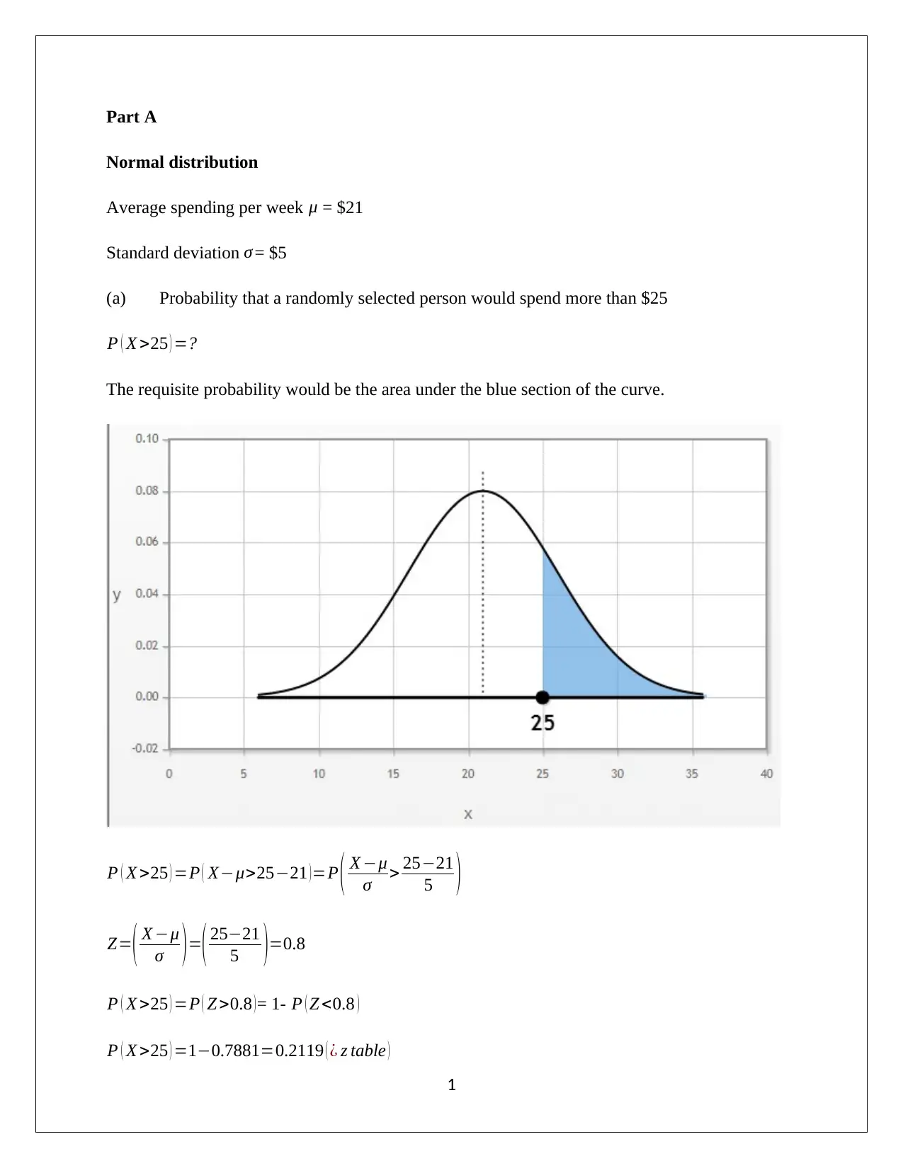
(a) Probability that a randomly selected person would spend more than $25
P ( X >25 ) =?
The requisite probability would be the area under the blue section of the curve.
P ( X >25 ) =P ( X−μ>25−21 )=P ( X −μ
σ > 25−21
5 )
Z=( X −μ
σ )=( 25−21
5 )=0.8
P ( X >25 ) =P ( Z >0.8 )= 1- P ( Z <0.8 )
P ( X >25 ) =1−0.7881=0.2119 ( ¿ z table )
1
Therefore, the probability that a randomly selected person would spend more than $25 is 0.2119.
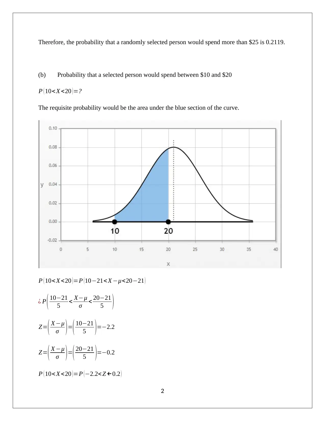
(b) Probability that a selected person would spend between $10 and $20
P ( 10< X <20 ) =?
The requisite probability would be the area under the blue section of the curve.
P ( 10< X <20 )=P (10−21<X −μ<20−21 )
¿ P ( 10−21
5 < X−μ
σ < 20−21
5 )
Z=( X −μ
σ )=( 10−21
5 )=−2.2
Z=( X −μ
σ ) =( 20−21
5 )=−0.2
P ( 10< X <20 )=P (−2.2< Z ←0.2 )
2
⊘ This is a preview!⊘
Do you want full access?
Subscribe today to unlock all pages.

Trusted by 1+ million students worldwide
P ( 10< X <20 )=P (−2.2< Z ←0.2 )=0.4068 ( ¿ z table )
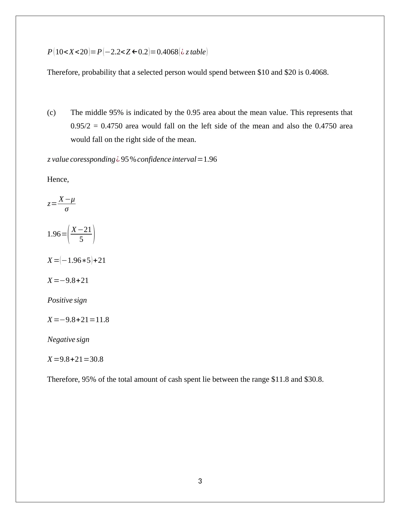
Therefore, probability that a selected person would spend between $10 and $20 is 0.4068.
(c) The middle 95% is indicated by the 0.95 area about the mean value. This represents that
0.95/2 = 0.4750 area would fall on the left side of the mean and also the 0.4750 area
would fall on the right side of the mean.
z value coressponding ¿ 95 % confidence interval=1.96
Hence,
z= X −μ
σ
1.96=( X −21
5 )
X = (−1.96∗5 ) +21
X =−9.8+21
Positive sign
X =−9.8+21=11.8
Negative sign
X =9.8+21=30.8
Therefore, 95% of the total amount of cash spent lie between the range $11.8 and $30.8.
3
Paraphrase This Document
Need a fresh take? Get an instant paraphrase of this document with our AI Paraphraser
Part B
Introduction
The data file regarding prevalent property taxes per capita in the various states has been
presented. The objective of this report is to analyse the given data and determine if it is
appropriate to conclude that the given data is normally distributed or not. This may be served in a
plethora of ways such as through boxplot, histogram or normal probability plot construction
(Bryc 2012, 96). Additionally, it may also be possible to compare whether the given data tends to
comply with the various characteristics that are usually associated with any data that tends to
follow a normal distribution (Elzey 2001, 79). One of the properties in this regard is that the
various measures of central tendency must coincide. This is related to the symmetric nature of
the normal curve which is also indicative of the skew being zero (Bearver 2012, 95). Presence of
skew leads to tail either on the right or left which in turn would highlight the non-normality of
the concerned data (Bulmer 2012, 89). Additionally, there are certain theoretical properties
particularly in relation to the particular distribution of data which must be exhibited which is
expected from a normal distribution. Hence, comparison of the actual properties of the given data
with the expected theoretical properties may be carried out which would enable in understanding
whether normality persists or not for the given data (Weiers 2010, 115). The findings of the
various techniques applied would be concluded at the end along with the underlying distribution
of the variable of interest i.e. property tax per capita.
Analysis
For analysing the given data, various techniques have been implemented and presented below
along with the potential implications of the same for normality.
(a) Construction of box plot
4
0
0.1
0.2
0.3
0.4
0.5
0.6
0.7
0.8
0.9
1
Box Plot - Property Taxes Per Capita ($)
Five number summary
Comment on Box Plot
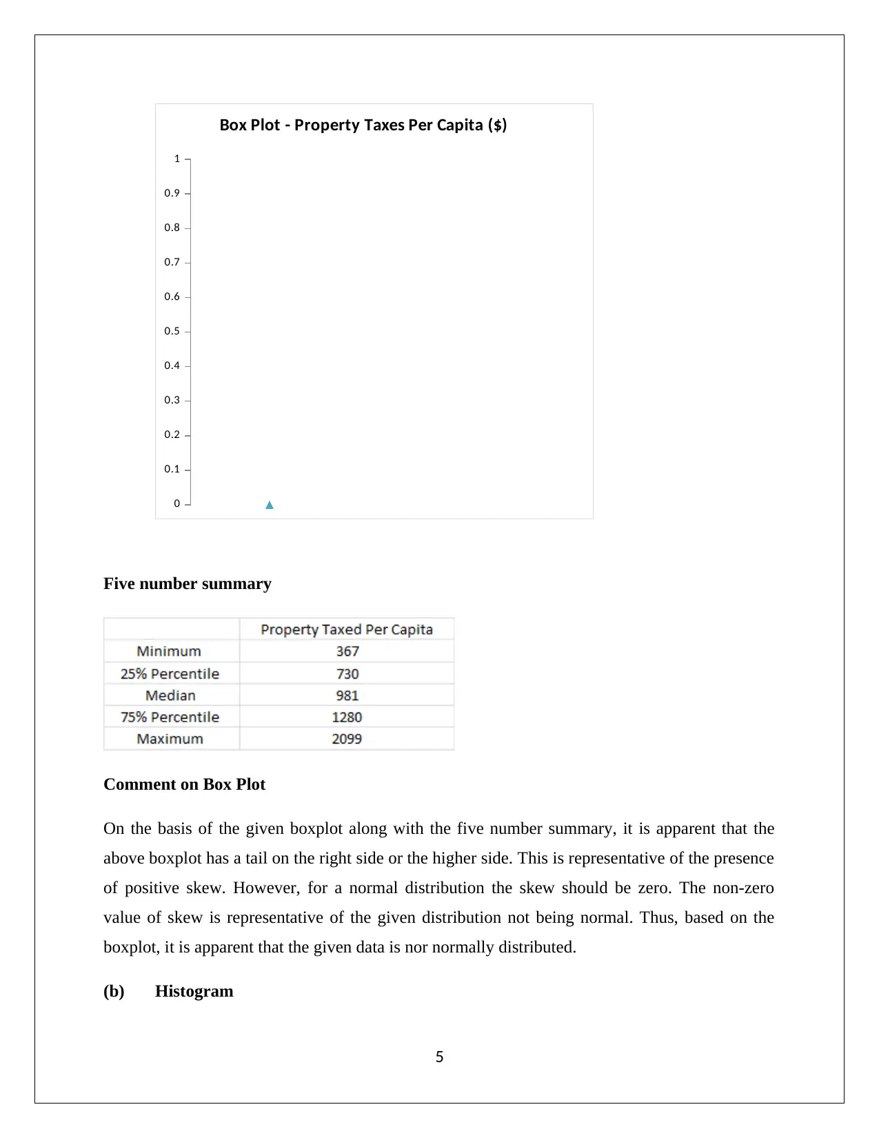
On the basis of the given boxplot along with the five number summary, it is apparent that the
above boxplot has a tail on the right side or the higher side. This is representative of the presence
of positive skew. However, for a normal distribution the skew should be zero. The non-zero
value of skew is representative of the given distribution not being normal. Thus, based on the
boxplot, it is apparent that the given data is nor normally distributed.
(b) Histogram
5
⊘ This is a preview!⊘
Do you want full access?
Subscribe today to unlock all pages.

Trusted by 1+ million students worldwide
0 to 713 713 to 1060 1060 to 1406 1406 to 1753 1753 or more
0
2
4
6
8
10
12
14
16
18
20
Histogram-Property Taxes Per Capita ($)
Property taxes per capita ($)
Frequency
Comment on Histogram
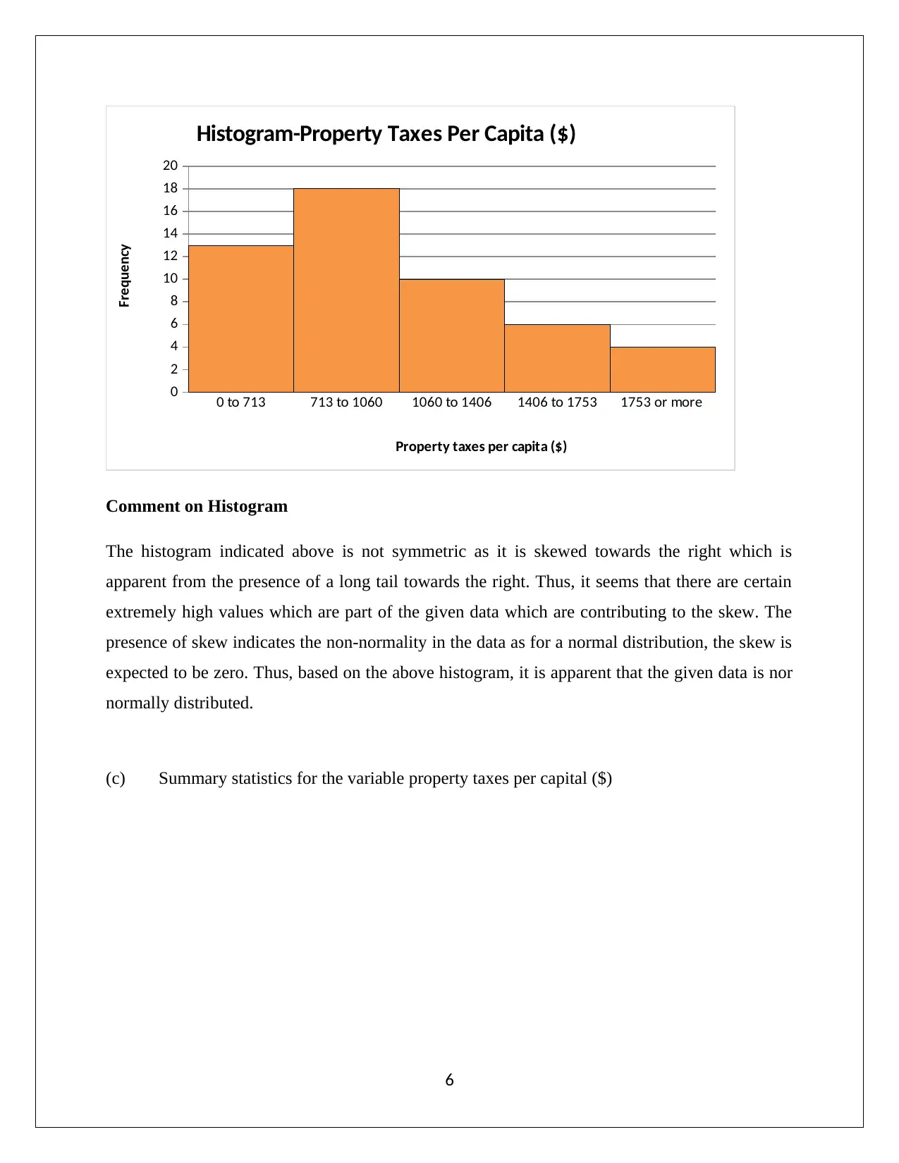
The histogram indicated above is not symmetric as it is skewed towards the right which is
apparent from the presence of a long tail towards the right. Thus, it seems that there are certain
extremely high values which are part of the given data which are contributing to the skew. The
presence of skew indicates the non-normality in the data as for a normal distribution, the skew is
expected to be zero. Thus, based on the above histogram, it is apparent that the given data is nor
normally distributed.
(c) Summary statistics for the variable property taxes per capital ($)
6
Paraphrase This Document
Need a fresh take? Get an instant paraphrase of this document with our AI Paraphraser
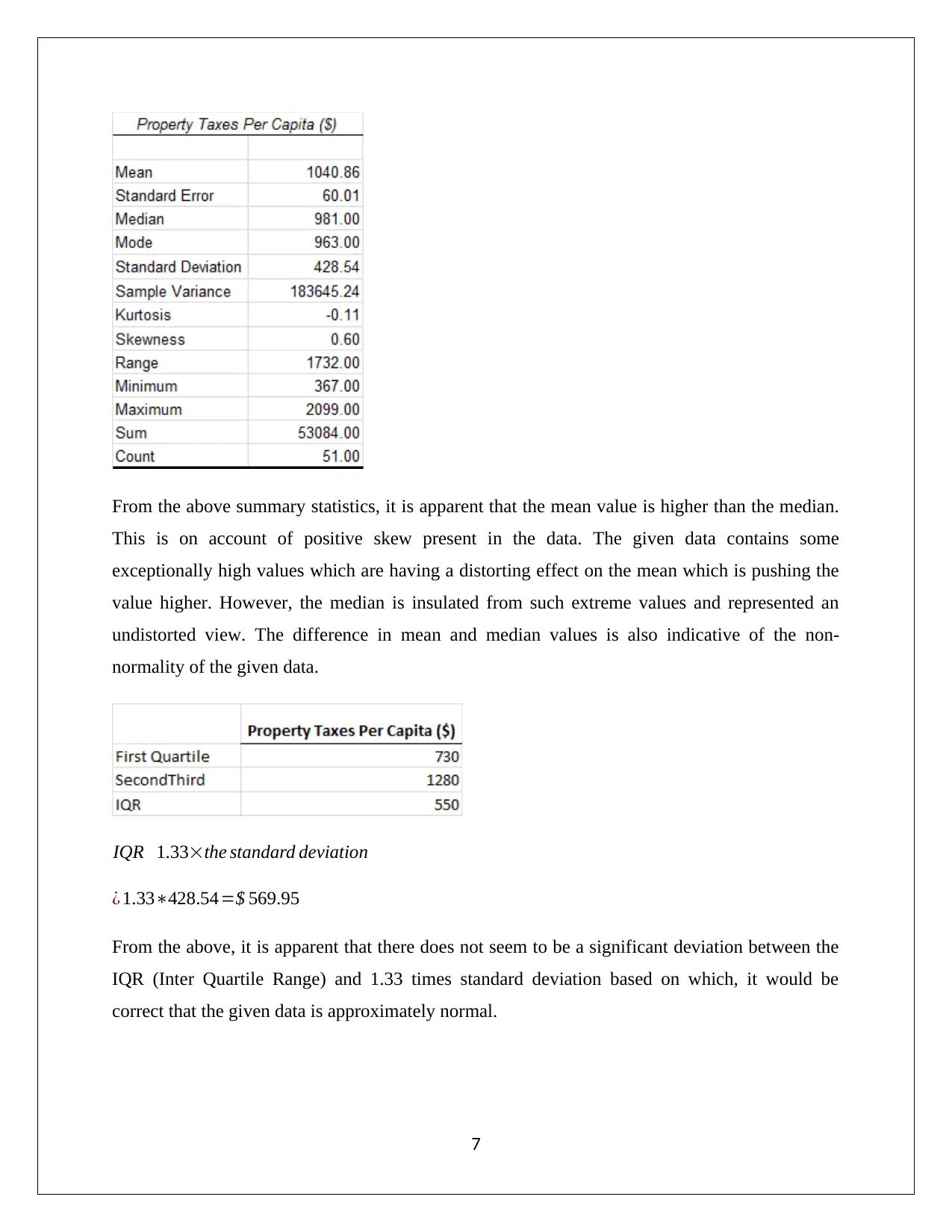
From the above summary statistics, it is apparent that the mean value is higher than the median.
This is on account of positive skew present in the data. The given data contains some
exceptionally high values which are having a distorting effect on the mean which is pushing the
value higher. However, the median is insulated from such extreme values and represented an
undistorted view. The difference in mean and median values is also indicative of the non-
normality of the given data.
IQR 1.33×the standard deviation
¿ 1.33∗428.54=$ 569.95
From the above, it is apparent that there does not seem to be a significant deviation between the
IQR (Inter Quartile Range) and 1.33 times standard deviation based on which, it would be
correct that the given data is approximately normal.
7
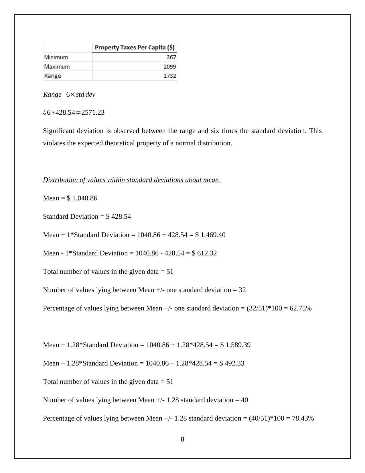
Range 6×std dev
¿ 6∗428.54=2571.23
Significant deviation is observed between the range and six times the standard deviation. This
violates the expected theoretical property of a normal distribution.
Distribution of values within standard deviations about mean
Mean = $ 1,040.86
Standard Deviation = $ 428.54
Mean + 1*Standard Deviation = 1040.86 + 428.54 = $ 1,469.40
Mean - 1*Standard Deviation = 1040.86 - 428.54 = $ 612.32
Total number of values in the given data = 51
Number of values lying between Mean +/- one standard deviation = 32
Percentage of values lying between Mean +/- one standard deviation = (32/51)*100 = 62.75%
Mean + 1.28*Standard Deviation = 1040.86 + 1.28*428.54 = $ 1,589.39
Mean – 1.28*Standard Deviation = 1040.86 – 1.28*428.54 = $ 492.33
Total number of values in the given data = 51
Number of values lying between Mean +/- 1.28 standard deviation = 40
Percentage of values lying between Mean +/- 1.28 standard deviation = (40/51)*100 = 78.43%
8
⊘ This is a preview!⊘
Do you want full access?
Subscribe today to unlock all pages.

Trusted by 1+ million students worldwide
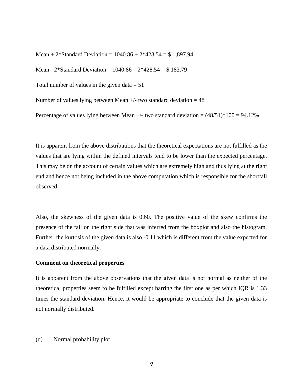
Mean + 2*Standard Deviation = 1040.86 + 2*428.54 = $ 1,897.94
Mean - 2*Standard Deviation = 1040.86 – 2*428.54 = $ 183.79
Total number of values in the given data = 51
Number of values lying between Mean +/- two standard deviation = 48
Percentage of values lying between Mean +/- two standard deviation = (48/51)*100 = 94.12%
It is apparent from the above distributions that the theoretical expectations are not fulfilled as the
values that are lying within the defined intervals tend to be lower than the expected percentage.
This may be on the account of certain values which are extremely high and thus lying at the right
end and hence not being included in the above computation which is responsible for the shortfall
observed.
Also, the skewness of the given data is 0.60. The positive value of the skew confirms the
presence of the tail on the right side that was inferred from the boxplot and also the histogram.
Further, the kurtosis of the given data is also -0.11 which is different from the value expected for
a data distributed normally.
Comment on theoretical properties
It is apparent from the above observations that the given data is not normal as neither of the
theoretical properties seem to be fulfilled except barring the first one as per which IQR is 1.33
times the standard deviation. Hence, it would be appropriate to conclude that the given data is
not normally distributed.
(d) Normal probability plot
9
Paraphrase This Document
Need a fresh take? Get an instant paraphrase of this document with our AI Paraphraser
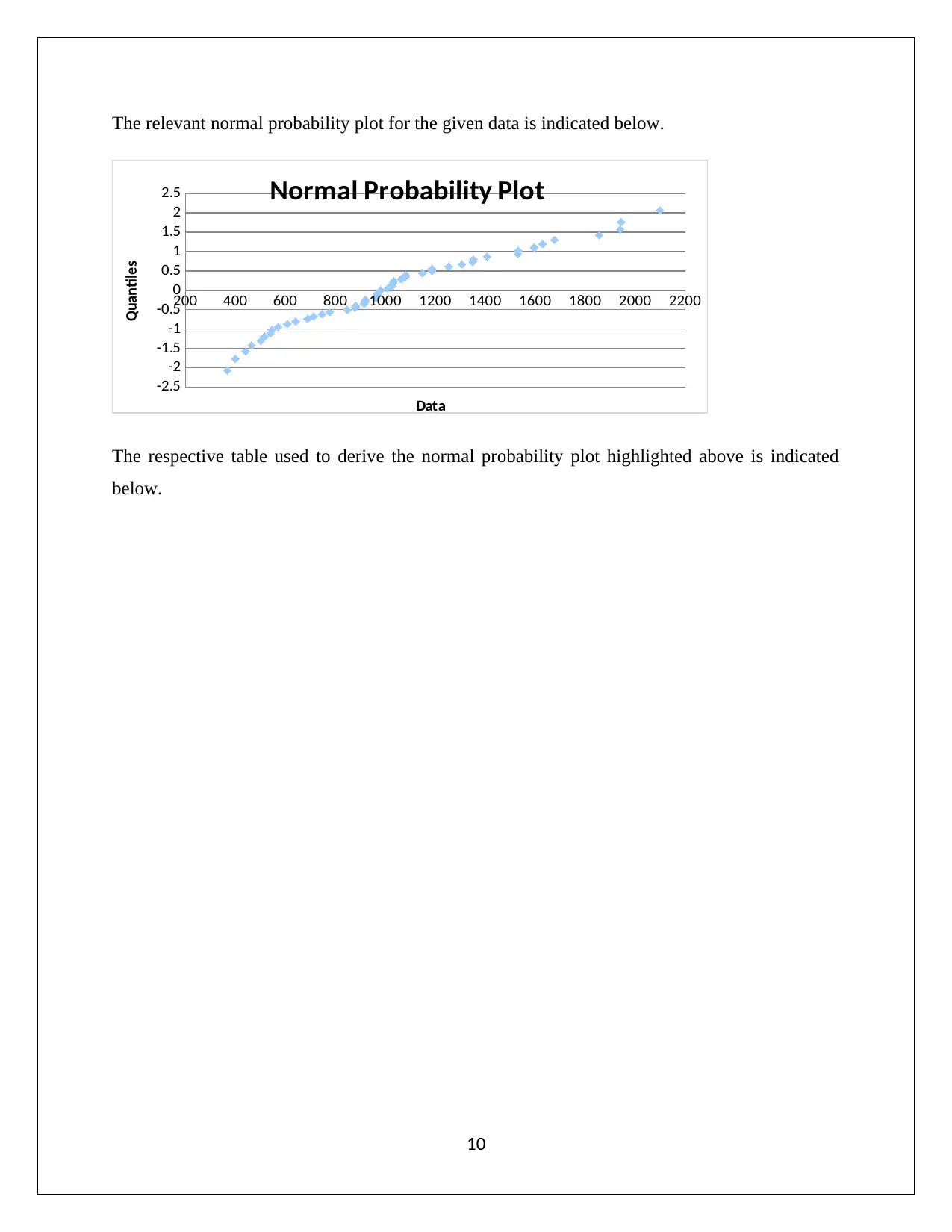
The relevant normal probability plot for the given data is indicated below.
200 400 600 800 1000 1200 1400 1600 1800 2000 2200
-2.5
-2
-1.5
-1
-0.5
0
0.5
1
1.5
2
2.5 Normal Probability Plot
Data
Quantiles
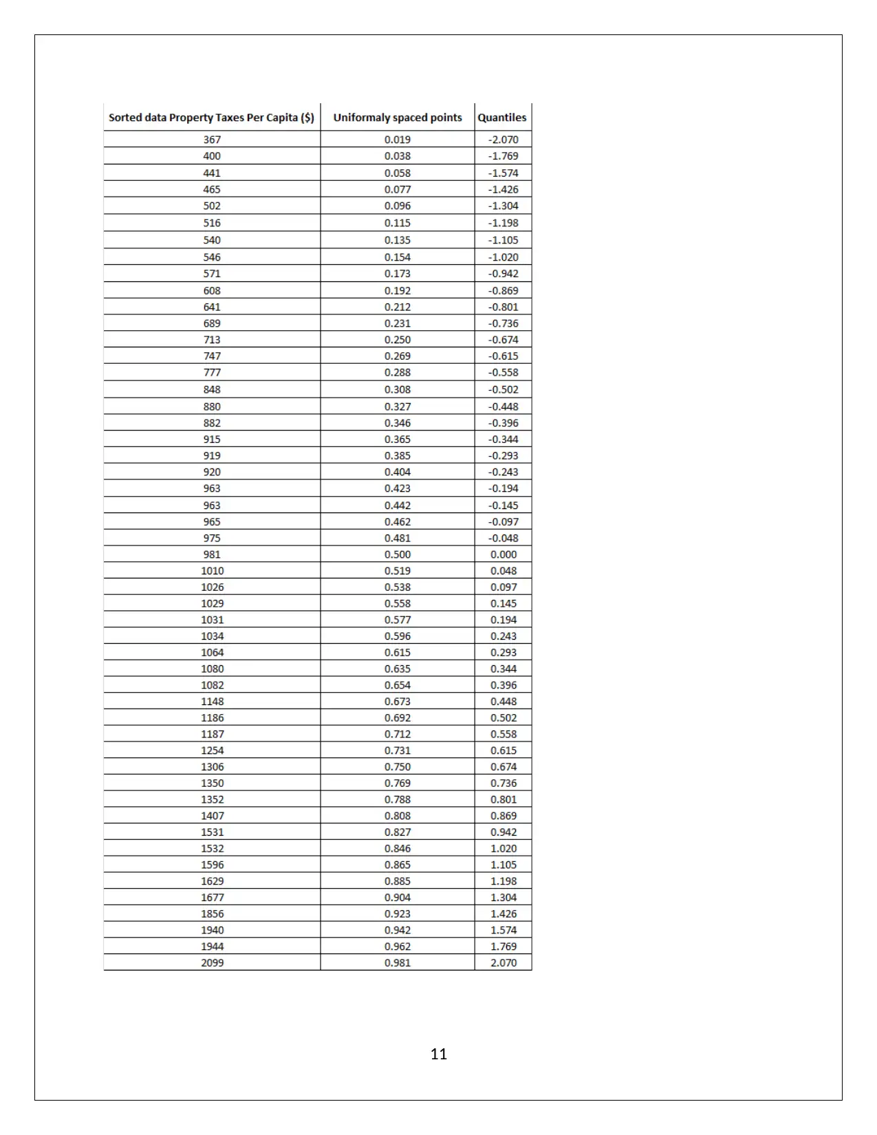
The respective table used to derive the normal probability plot highlighted above is indicated
below.
10
200 400 600 800 1000 1200 1400 1600 1800 2000 2200
-2.5
-2
-1.5
-1
-0.5
0
0.5
1
1.5
2
2.5 Normal Probability Plot
Data
Quantiles
The respective table used to derive the normal probability plot highlighted above is indicated
below.
10
11
⊘ This is a preview!⊘
Do you want full access?
Subscribe today to unlock all pages.

Trusted by 1+ million students worldwide
1 out of 14
Related Documents
Your All-in-One AI-Powered Toolkit for Academic Success.
+13062052269
info@desklib.com
Available 24*7 on WhatsApp / Email
![[object Object]](/_next/static/media/star-bottom.7253800d.svg)
Unlock your academic potential
Copyright © 2020–2026 A2Z Services. All Rights Reserved. Developed and managed by ZUCOL.


