Analysis of TV Viewership Behaviors Among NSW Residents, BEA603, 2019
VerifiedAdded on 2023/01/19
|14
|2586
|48
Report
AI Summary
This report presents an analysis of TV viewership behaviors among residents of New South Wales, Australia, based on a survey of 100 respondents. The study explores various aspects of TV viewing habits, including the frequency of viewing, preferred programs (soaps, news, etc.), time of day, and the relationship between gender and program preferences. The analysis includes descriptive statistics (frequencies, percentages), cross-tabulations, pie charts, side-by-side bar charts, scatter plots, and correlation coefficients to visualize and interpret the data. A key finding is the significant association between gender and the type of TV programs watched, with females showing a preference for soaps. The study also examines the joint probability of watching soap operas during specific time slots and tests hypotheses regarding differences in viewing time between genders, revealing that female respondents tend to spend more time watching TV. The report concludes with business implications, limitations of the study, and suggestions for future research, emphasizing the importance of understanding audience behavior for media houses and advertising purposes.
Analysis of TV viewership behaviors among residents of New South Wales
Statistics
Student Name:
Instructor Name:
Course Number:
14 April 2019
Statistics
Student Name:
Instructor Name:
Course Number:
14 April 2019
Paraphrase This Document
Need a fresh take? Get an instant paraphrase of this document with our AI Paraphraser
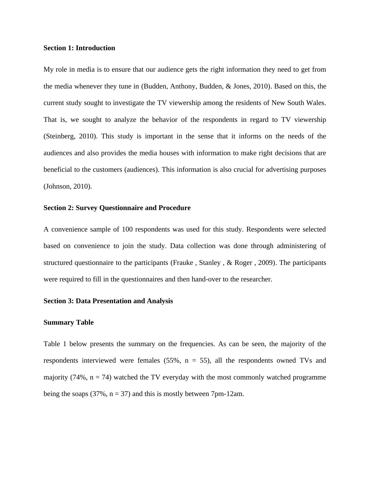
Section 1: Introduction
My role in media is to ensure that our audience gets the right information they need to get from
the media whenever they tune in (Budden, Anthony, Budden, & Jones, 2010). Based on this, the
current study sought to investigate the TV viewership among the residents of New South Wales.
That is, we sought to analyze the behavior of the respondents in regard to TV viewership
(Steinberg, 2010). This study is important in the sense that it informs on the needs of the
audiences and also provides the media houses with information to make right decisions that are
beneficial to the customers (audiences). This information is also crucial for advertising purposes
(Johnson, 2010).
Section 2: Survey Questionnaire and Procedure
A convenience sample of 100 respondents was used for this study. Respondents were selected
based on convenience to join the study. Data collection was done through administering of
structured questionnaire to the participants (Frauke , Stanley , & Roger , 2009). The participants
were required to fill in the questionnaires and then hand-over to the researcher.
Section 3: Data Presentation and Analysis
Summary Table
Table 1 below presents the summary on the frequencies. As can be seen, the majority of the
respondents interviewed were females (55%, n = 55), all the respondents owned TVs and
majority (74%, n = 74) watched the TV everyday with the most commonly watched programme
being the soaps (37%, n = 37) and this is mostly between 7pm-12am.

Table 1: Summary table for the frequencies
Characteristics Frequency (n) Percent (%)
Gender
Male 55 55.0
Female 45 45.0
Total 100 100.0
TV ownership
Yes 100 100.0
No 0 0.0
Total 100 100.0
Frequency of watching TV
Everyday 74 74.0
Every other day 14 14.0
Once a week 6 6.0
Once every 2 weeks 6 6.0
Total 100 100.0
Programme most commonly watched
Soaps 37 37.0
Reality 15 15.0
News 14 14.0
Drama 8 8.0
Comedy 8 8.0
Sports 18 18.0
Total 100 100.0
Additions to the terrestrial TV
Sky 27 27.0
Virgin 12 12.0
Freeview 18 18.0
Sky Go 16 16.0
Apple TV 11 11.0
Amazon Prime 16 16.0
Total 100 100.0
Days of the week when watch TV the most
Mondays 7 7.0
Tuesdays 9 9.0
Wednesdays 8 8.0
Thursdays 9 9.0
Fridays 11 11.0
Saturdays 25 25.0
Sundays 31 31.0
Total 100 100.0
⊘ This is a preview!⊘
Do you want full access?
Subscribe today to unlock all pages.
Trusted by 1+ million students worldwide
Days of the week when watch TV the least
Mondays 46 46.0
Tuesdays 18 18.0
Wednesdays 6 6.0
Thursdays 8 8.0
Fridays 1 1.0
Saturdays 6 6.0
Sundays 15 15.0
Total 100 100.0
Time usually watch TV shows
7am – 12pm 19 19.0
12pm – 3pm 11 11.0
4pm – 7pm 9 9.0
7pm – 9pm 26 26.0
9pm – 12am 35 35.0
Total 100 100.0
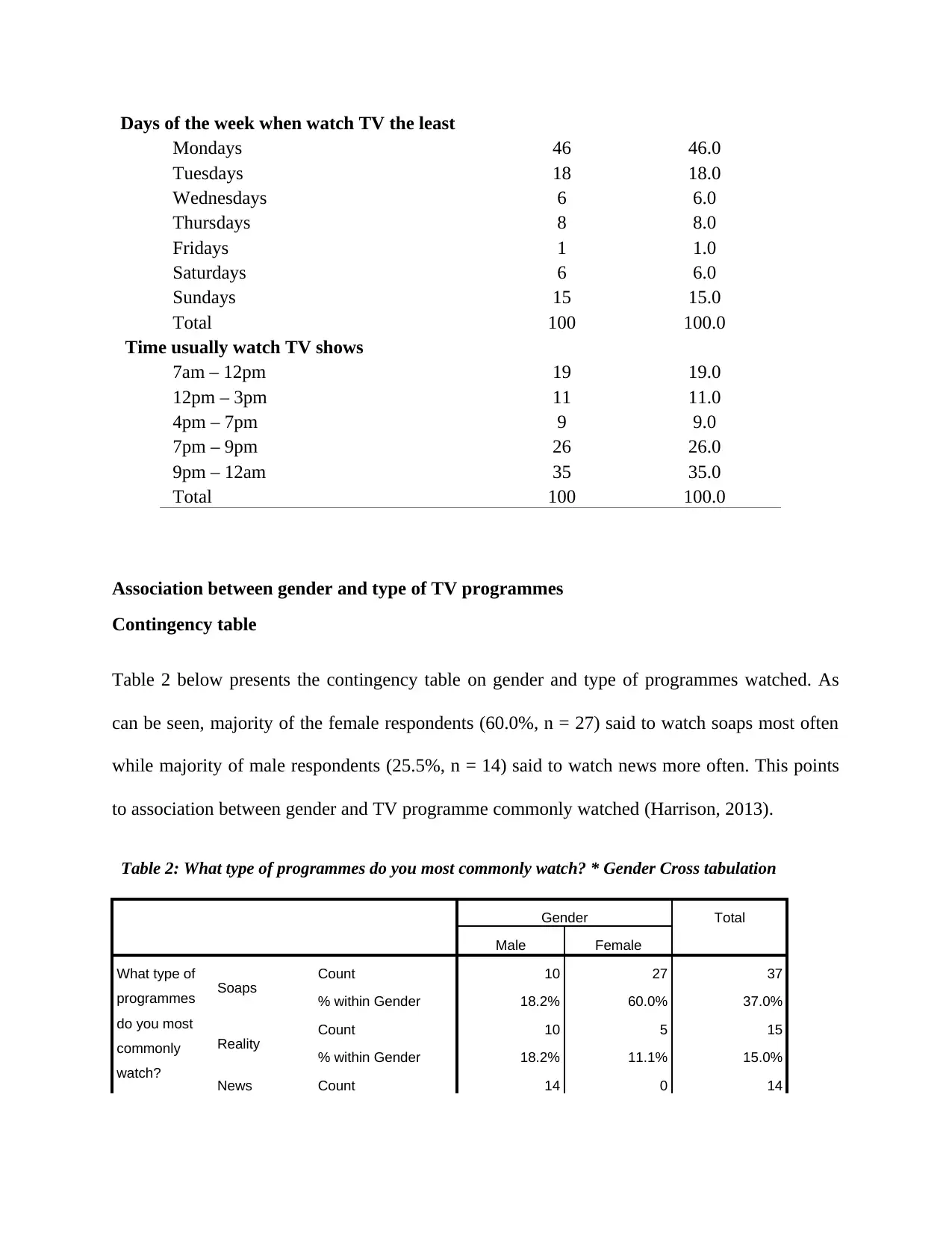
Association between gender and type of TV programmes
Contingency table
Table 2 below presents the contingency table on gender and type of programmes watched. As
can be seen, majority of the female respondents (60.0%, n = 27) said to watch soaps most often
while majority of male respondents (25.5%, n = 14) said to watch news more often. This points
to association between gender and TV programme commonly watched (Harrison, 2013).
Table 2: What type of programmes do you most commonly watch? * Gender Cross tabulation
Gender Total
Male Female
What type of
programmes
do you most
commonly
watch?
Soaps Count 10 27 37
% within Gender 18.2% 60.0% 37.0%
Reality Count 10 5 15
% within Gender 18.2% 11.1% 15.0%
News Count 14 0 14
Mondays 46 46.0
Tuesdays 18 18.0
Wednesdays 6 6.0
Thursdays 8 8.0
Fridays 1 1.0
Saturdays 6 6.0
Sundays 15 15.0
Total 100 100.0
Time usually watch TV shows
7am – 12pm 19 19.0
12pm – 3pm 11 11.0
4pm – 7pm 9 9.0
7pm – 9pm 26 26.0
9pm – 12am 35 35.0
Total 100 100.0
Association between gender and type of TV programmes
Contingency table
Table 2 below presents the contingency table on gender and type of programmes watched. As
can be seen, majority of the female respondents (60.0%, n = 27) said to watch soaps most often
while majority of male respondents (25.5%, n = 14) said to watch news more often. This points
to association between gender and TV programme commonly watched (Harrison, 2013).
Table 2: What type of programmes do you most commonly watch? * Gender Cross tabulation
Gender Total
Male Female
What type of
programmes
do you most
commonly
watch?
Soaps Count 10 27 37
% within Gender 18.2% 60.0% 37.0%
Reality Count 10 5 15
% within Gender 18.2% 11.1% 15.0%
News Count 14 0 14
Paraphrase This Document
Need a fresh take? Get an instant paraphrase of this document with our AI Paraphraser
% within Gender 25.5% 0.0% 14.0%
Drama Count 4 4 8
% within Gender 7.3% 8.9% 8.0%
Comedy Count 4 4 8
% within Gender 7.3% 8.9% 8.0%
Sports Count 13 5 18
% within Gender 23.6% 11.1% 18.0%
Total Count 55 45 100
% within Gender 100.0% 100.0% 100.0%
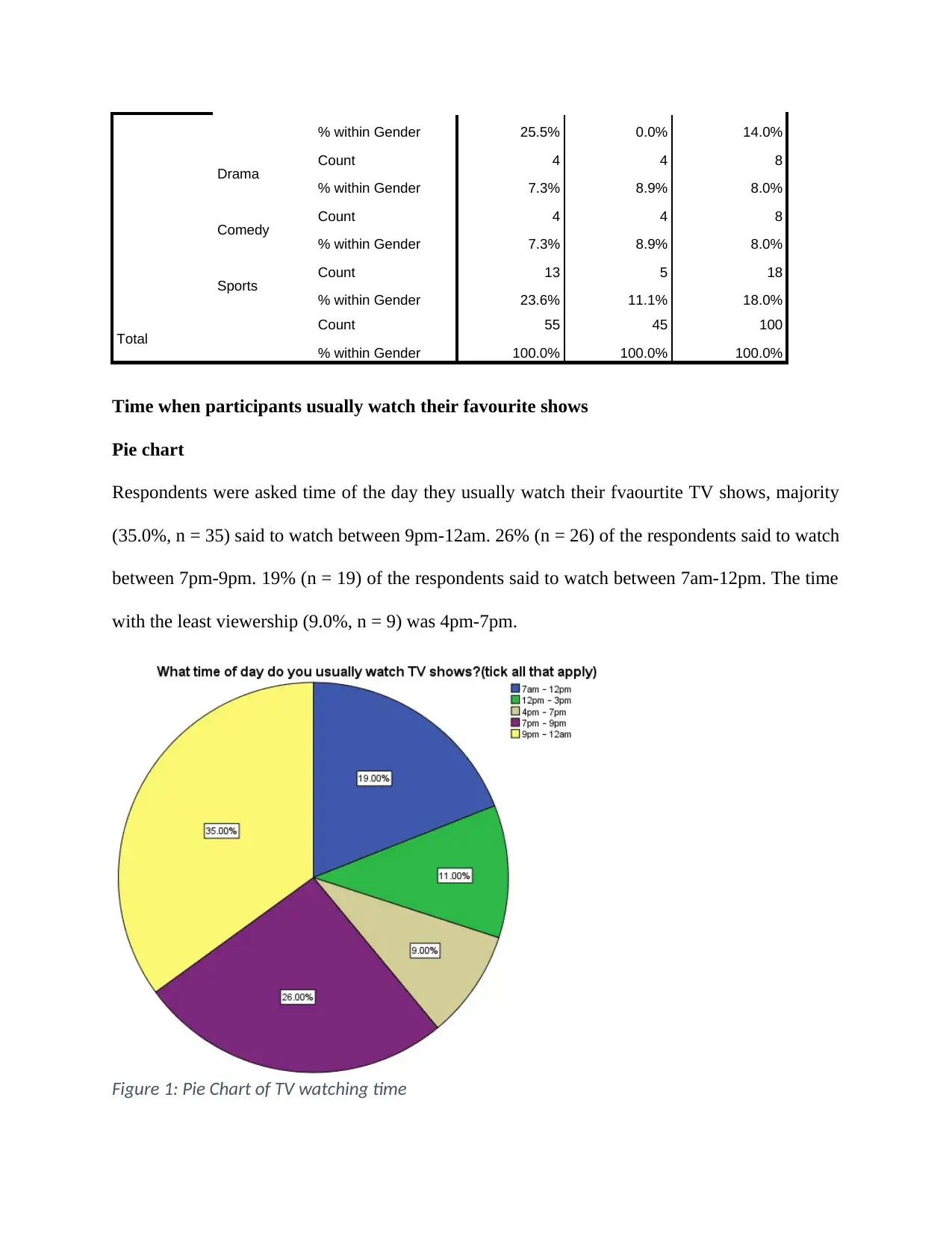
Time when participants usually watch their favourite shows
Pie chart
Respondents were asked time of the day they usually watch their fvaourtite TV shows, majority
(35.0%, n = 35) said to watch between 9pm-12am. 26% (n = 26) of the respondents said to watch
between 7pm-9pm. 19% (n = 19) of the respondents said to watch between 7am-12pm. The time
with the least viewership (9.0%, n = 9) was 4pm-7pm.
Figure 1: Pie Chart of TV watching time
Drama Count 4 4 8
% within Gender 7.3% 8.9% 8.0%
Comedy Count 4 4 8
% within Gender 7.3% 8.9% 8.0%
Sports Count 13 5 18
% within Gender 23.6% 11.1% 18.0%
Total Count 55 45 100
% within Gender 100.0% 100.0% 100.0%
Time when participants usually watch their favourite shows
Pie chart
Respondents were asked time of the day they usually watch their fvaourtite TV shows, majority
(35.0%, n = 35) said to watch between 9pm-12am. 26% (n = 26) of the respondents said to watch
between 7pm-9pm. 19% (n = 19) of the respondents said to watch between 7am-12pm. The time
with the least viewership (9.0%, n = 9) was 4pm-7pm.
Figure 1: Pie Chart of TV watching time
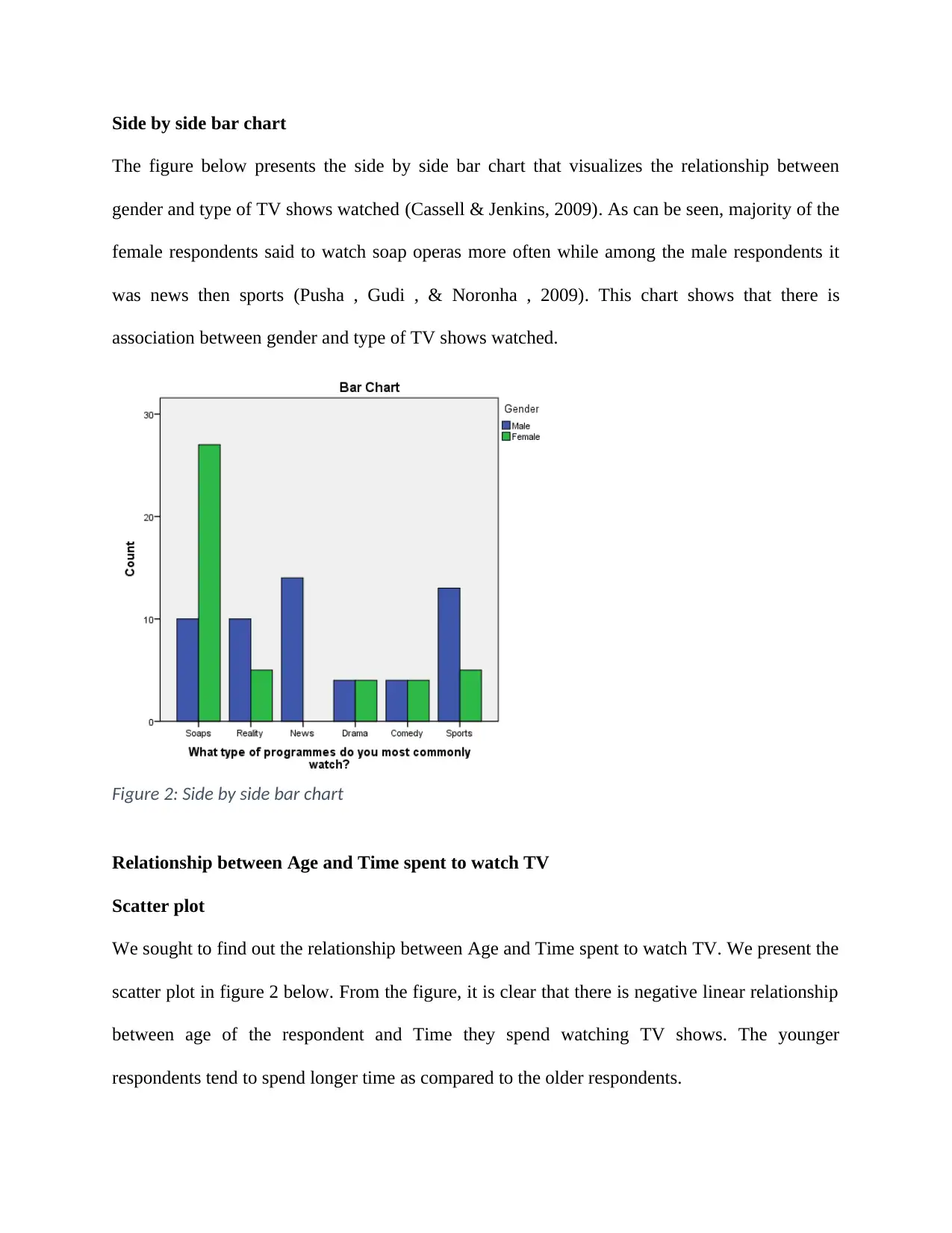
Side by side bar chart
The figure below presents the side by side bar chart that visualizes the relationship between
gender and type of TV shows watched (Cassell & Jenkins, 2009). As can be seen, majority of the
female respondents said to watch soap operas more often while among the male respondents it
was news then sports (Pusha , Gudi , & Noronha , 2009). This chart shows that there is
association between gender and type of TV shows watched.
Figure 2: Side by side bar chart
Relationship between Age and Time spent to watch TV
Scatter plot
We sought to find out the relationship between Age and Time spent to watch TV. We present the
scatter plot in figure 2 below. From the figure, it is clear that there is negative linear relationship
between age of the respondent and Time they spend watching TV shows. The younger
respondents tend to spend longer time as compared to the older respondents.
⊘ This is a preview!⊘
Do you want full access?
Subscribe today to unlock all pages.
Trusted by 1+ million students worldwide
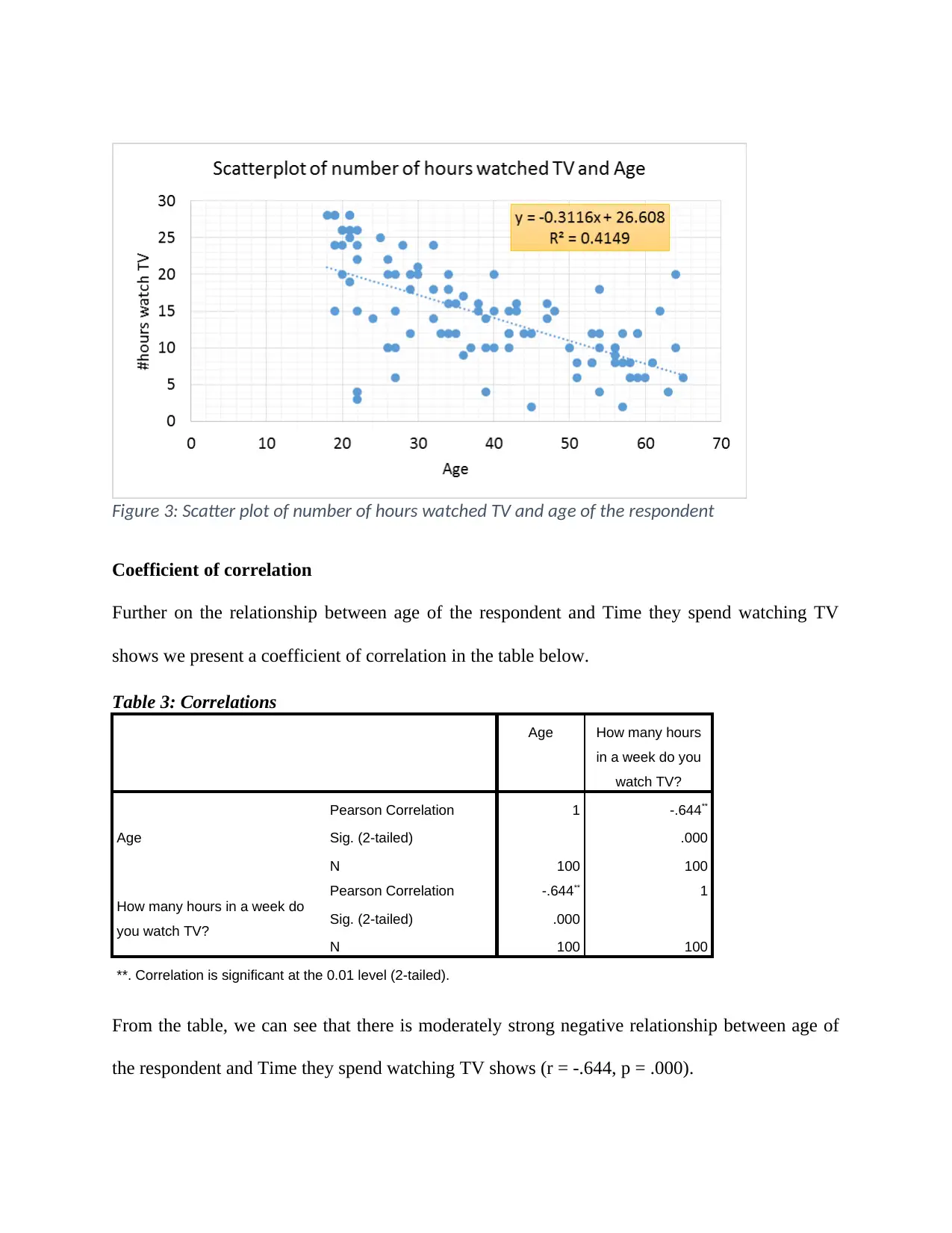
Figure 3: Scatter plot of number of hours watched TV and age of the respondent
Coefficient of correlation
Further on the relationship between age of the respondent and Time they spend watching TV
shows we present a coefficient of correlation in the table below.
Table 3: Correlations
Age How many hours
in a week do you
watch TV?
Age
Pearson Correlation 1 -.644**
Sig. (2-tailed) .000
N 100 100
How many hours in a week do
you watch TV?
Pearson Correlation -.644** 1
Sig. (2-tailed) .000
N 100 100
**. Correlation is significant at the 0.01 level (2-tailed).
From the table, we can see that there is moderately strong negative relationship between age of
the respondent and Time they spend watching TV shows (r = -.644, p = .000).
Paraphrase This Document
Need a fresh take? Get an instant paraphrase of this document with our AI Paraphraser
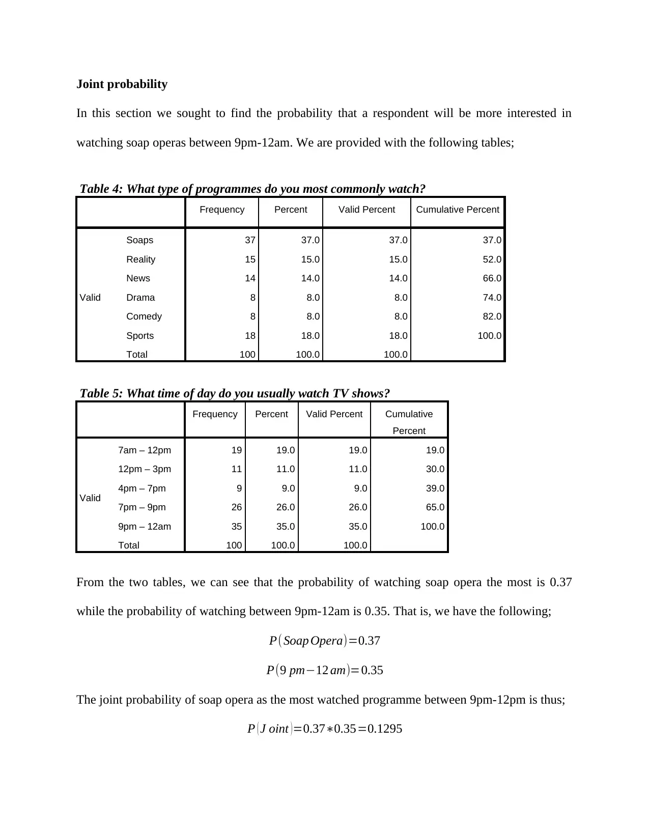
Joint probability
In this section we sought to find the probability that a respondent will be more interested in
watching soap operas between 9pm-12am. We are provided with the following tables;
Table 4: What type of programmes do you most commonly watch?
Frequency Percent Valid Percent Cumulative Percent
Valid
Soaps 37 37.0 37.0 37.0
Reality 15 15.0 15.0 52.0
News 14 14.0 14.0 66.0
Drama 8 8.0 8.0 74.0
Comedy 8 8.0 8.0 82.0
Sports 18 18.0 18.0 100.0
Total 100 100.0 100.0
Table 5: What time of day do you usually watch TV shows?
Frequency Percent Valid Percent Cumulative
Percent
Valid
7am – 12pm 19 19.0 19.0 19.0
12pm – 3pm 11 11.0 11.0 30.0
4pm – 7pm 9 9.0 9.0 39.0
7pm – 9pm 26 26.0 26.0 65.0
9pm – 12am 35 35.0 35.0 100.0
Total 100 100.0 100.0
From the two tables, we can see that the probability of watching soap opera the most is 0.37
while the probability of watching between 9pm-12am is 0.35. That is, we have the following;
P( Soap Opera)=0.37
P(9 pm−12 am)=0.35
The joint probability of soap opera as the most watched programme between 9pm-12pm is thus;
P ( J oint )=0.37∗0.35=0.1295
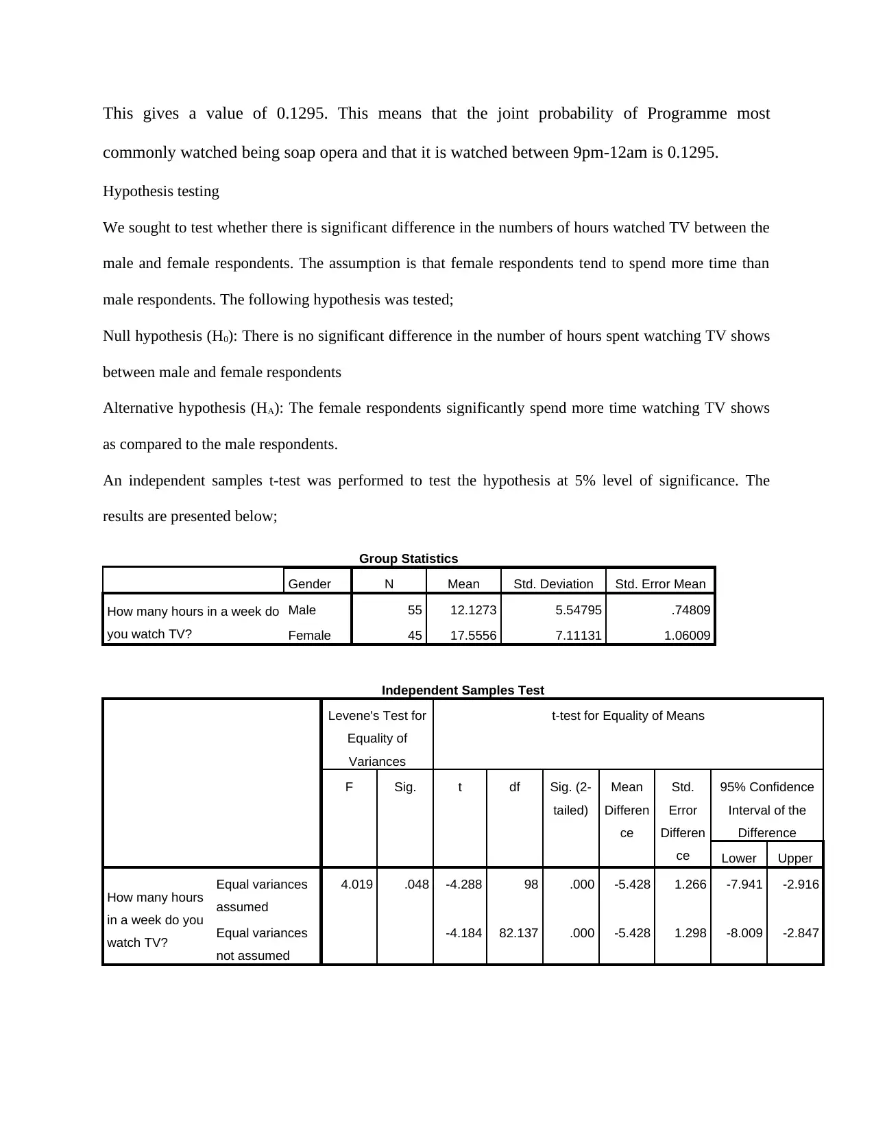
This gives a value of 0.1295. This means that the joint probability of Programme most
commonly watched being soap opera and that it is watched between 9pm-12am is 0.1295.
Hypothesis testing
We sought to test whether there is significant difference in the numbers of hours watched TV between the
male and female respondents. The assumption is that female respondents tend to spend more time than
male respondents. The following hypothesis was tested;
Null hypothesis (H0): There is no significant difference in the number of hours spent watching TV shows
between male and female respondents
Alternative hypothesis (HA): The female respondents significantly spend more time watching TV shows
as compared to the male respondents.
An independent samples t-test was performed to test the hypothesis at 5% level of significance. The
results are presented below;
Group Statistics
Gender N Mean Std. Deviation Std. Error Mean
How many hours in a week do
you watch TV?
Male 55 12.1273 5.54795 .74809
Female 45 17.5556 7.11131 1.06009
Independent Samples Test
Levene's Test for
Equality of
Variances
t-test for Equality of Means
F Sig. t df Sig. (2-
tailed)
Mean
Differen
ce
Std.
Error
Differen
ce
95% Confidence
Interval of the
Difference
Lower Upper
How many hours
in a week do you
watch TV?
Equal variances
assumed
4.019 .048 -4.288 98 .000 -5.428 1.266 -7.941 -2.916
Equal variances
not assumed
-4.184 82.137 .000 -5.428 1.298 -8.009 -2.847
⊘ This is a preview!⊘
Do you want full access?
Subscribe today to unlock all pages.
Trusted by 1+ million students worldwide
An independent samples t-test was performed to compare the mean number of hours spent
watching TV shows between the male and the female respondents. Results showed that the
female respondents (M = 17.56, SD = 7.11, N = 45) significantly spent more hours watching TV
shows as compared to the male respondents (M = 12.13, SD = 5.55, N = 55), t (98) = -4.288, p
< .05, two-tailed. The difference of 5.428 showed a significant difference. Essentially results
showed that female respondents who took part in the study tend to spend longer hours watching
TV shows as compared to the male respondents (Beh, 2014).
Section 4: Conclusion
Business or policy decision making implications
The aim of this study was to analyze the behavior of the TV audiences. A sample of 100
participants took part in the study. Results that female respondents tend to spend more time
watching TV shows as compared to the male respondents. Results further revealed that there is
significant association between gender and type of TV shows watched. This findings are very
important for decision making as they inform the media houses on which TV shows to air at
what time so that they are able to meet the needs of their audiences.
Limitations of the study
The study was limited by a number of issues. These issues are listed below;
Small sample size; the sample size used for this study was small so not very good for
generalizations.
Data was only collected in one region, this could have biased results.
Non-random sampling; respondents were selected based on convenience method. This
could pose some bias to the results
Paraphrase This Document
Need a fresh take? Get an instant paraphrase of this document with our AI Paraphraser
Suggestions for future studies
Based on the limitations of this study, future study should try and improve by doing the
following;
Work on having a larger sample size. Future study should try and have a study with a
large sample size to ensure that the results are good for generalization
Have multiple regions as data collection points. Future study should focus on getting
data from various regions and not just from one region. This will help reduced bias
that may arise from collecting data from just one region.
Future study should ensure that the collection of data is done randomly. Non-random
sampling poses bias issues and this should not be the case for future studies.
References
Beh, E. J. (2014). Simple correspondence analysis: a bibliographic review. International
Statistical Review, 72(2), 257-284.
Budden, C., Anthony, J., Budden, M., & Jones, M. (2010). Managing the evolution of a
revolution: Marketing implications of internet media usage among college students.
College Teaching Methods & Styles Journal, 3(3), 7.
Cassell, J., & Jenkins, H. (2009). Chess for Girls? Feminism and Computer Games. Gender and
Computer Games, 5(3), 27.
Frauke , K., Stanley , P., & Roger , T. (2009). Social Desirability Bias in CATI, IVR, and Web
Surveys: The Effects of Mode and Question Sensitivity. Public Opinion Quarterly, 72(5),
847-865.
Harrison, K. (2013). Television Viewers' Ideal Body Proportions: the Case of the Curvaceously
Thin Woman. Sex Roles, 48(5), 255-264.
Johnson, C. (2010). Australia's highest-circulating advertising, marketing and media magazine.
Journal of Marketing, 5(2), 45-67.
Pusha , A., Gudi , R., & Noronha , S. (2009). Polar classification with correspondence analysis
for fault isolation. Journal of Process Control 19, 19(4), 656-663.
Steinberg, B. (2010). CW plans TV-sized commercial breaks for online viewing. Journal of
Advertising and Marketing, 10(5), 101-121.
Appendix
⊘ This is a preview!⊘
Do you want full access?
Subscribe today to unlock all pages.
Trusted by 1+ million students worldwide
1 out of 14
Your All-in-One AI-Powered Toolkit for Academic Success.
+13062052269
info@desklib.com
Available 24*7 on WhatsApp / Email
![[object Object]](/_next/static/media/star-bottom.7253800d.svg)
Unlock your academic potential
Copyright © 2020–2026 A2Z Services. All Rights Reserved. Developed and managed by ZUCOL.