Data Analysis and Forecasting for Transportation Costs Analysis

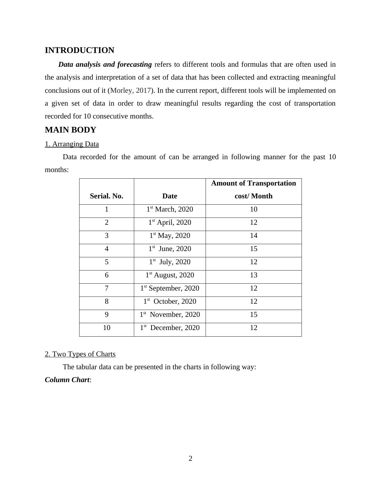
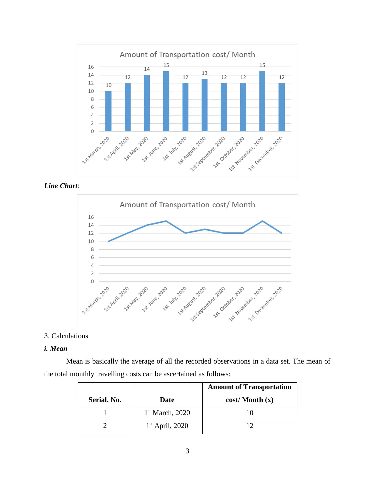
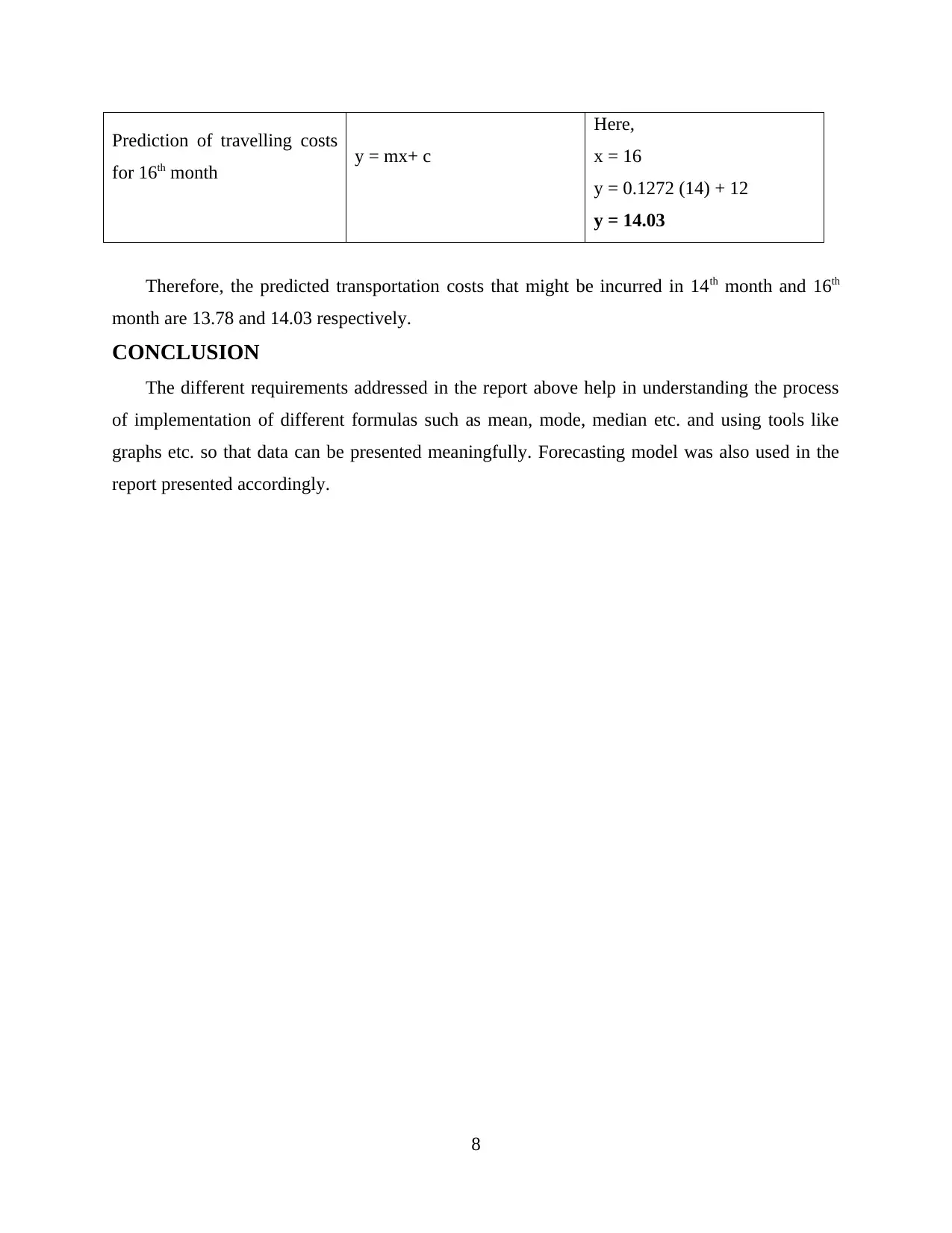
This report undertakes a detailed analysis of transportation cost data collected over ten months, employing various statistical techniques and forecasting models. The analysis begins with organizing the data and presenting it through column and line charts. Key statistical measures, including mean, median, mode, range, and standard deviation, are calculated to provide a comprehensive understanding of the data's central tendencies and variability. The report then constructs a linear forecasting model to predict future transportation costs, providing step-by-step calculations for the model's parameters and demonstrating its application to forecast costs for specific months. This assignment is a practical application of data analysis principles, offering insights into data interpretation, statistical computation, and predictive modeling.

DATA ANALYSIS AND
FORECASTING

TABLE OF CONTENTS
INTRODUCTION...........................................................................................................................2
MAIN BODY..................................................................................................................................2
1. Arranging Data........................................................................................................................2
2. Two Types of Charts...............................................................................................................2
3. Calculations.............................................................................................................................3
4. Forecasting model....................................................................................................................6
CONCLUSION................................................................................................................................8
REFERENCES................................................................................................................................9
1

INTRODUCTION
Data analysis and forecasting refers to different tools and formulas that are often used in
the analysis and interpretation of a set of data that has been collected and extracting meaningful
conclusions out of it (Morley, 2017). In the current report, different tools will be implemented on
a given set of data in order to draw meaningful results regarding the cost of transportation
recorded for 10 consecutive months.
MAIN BODY
1. Arranging Data
Data recorded for the amount of can be arranged in following manner for the past 10
months:
Serial. No. Date
Amount of Transportation
cost/ Month
1 1st March, 2020 10
2 1st April, 2020 12
3 1st May, 2020 14
4 1st June, 2020 15
5 1st July, 2020 12
6 1st August, 2020 13
7 1st September, 2020 12
8 1st October, 2020 12
9 1st November, 2020 15
10 1st December, 2020 12
2. Two Types of Charts
The tabular data can be presented in the charts in following way:
Column Chart:
2

Line Chart:
3. Calculations
i. Mean
Mean is basically the average of all the recorded observations in a data set. The mean of
the total monthly travelling costs can be ascertained as follows:
Serial. No. Date
Amount of Transportation
cost/ Month (x)
1 1st March, 2020 10
2 1st April, 2020 12
3

3 1st May, 2020 14
4 1st June, 2020 15
5 1st July, 2020 12
6 1st August, 2020 13
7 1st September, 2020 12
8 1st October, 2020 12
9 1st November, 2020 15
10 1st December, 2020 12
Total of transportation costs (∑x) 127
Total observations recorded (n) 10
Mean (∑x/ n) 12.7
This indicates that on an average, the transportation costs incurred in the past 10 months
in 12.7 or approximately 13.
ii. Median
Median is identified as the middle value of a set of observation (Soler-Hampejsek and
et.al., 2018). In order to ascertain the median of the recorded observations, they can be derived
through following steps:
1st step: Arranging observations in ascending order:
Serial. No. Date
Amount of Transportation
cost/ Month
1 1st March, 2020 10
2 1st April, 2020 12
3 1st July, 2020 12
4 1st September, 2020 12
5 1st October, 2020 12
6 1st December, 2020 12
7 1st August, 2020 13
8 1st May, 2020 14
9 1st June, 2020 15
10 1st November, 2020 15
4

Step 2: Using formula of (n + 1) / 2, median value can be identified as:
Median Value = (10 + 1) / 2 = 5.5 value
i.e. the middle of the 5th and 6th observation.
12+12 / 2 = 12 i.e. 12 is the median i.e. middle value for recorded observation.
iii. Mode
Since 12 can be easily identified as the most frequently recorded observation, it is clear
that this is the recorded mode for the given set of observation.
iv. Range
Range can be identified as the difference between the maximum and the minimum value
that has been recorded (Fisher and Marshall, 2019). In the present case of cost of transportation,
the range can be calculated as follows:
Range = Maximum – Minimum value = 15 – 10 = 5
v. Standard Deviation
The formula for calculation of standard deviation can be identified as:
Std. Deviation = Sq. root of Variance i.e.
σ =
and formula for variance is,
=
Where,
x = Individual observation value,
μ = Mean
∑ = Sum of
N = Number of observation
5

The variance for the recorded set where mean value is 12, as calculated earlier, can be
calculated as follows:
S.
No. Date Amount of Transportation cost/
Month (x) (x- μ) (x- μ) 2
1 1st March, 2020 10 -2 4
2 1st April, 2020 12 0 0
3 1st May, 2020 14 2 4
4 1st June, 2020 15 3 9
5 1st July, 2020 12 0 0
6 1st August, 2020 13 1 1
7 1st September, 2020 12 0 0
8 1st October, 2020 12 0 0
9 1st November, 2020 15 3 9
10 1st December, 2020 12 0 0
Total (∑) 27
Now, Variance can be evaluated as:
= 27 / 10 = 2.7
Therefore, standard deviation is:
σ = sq. root of 2.7 = 1.64
4. Forecasting model
The linear forecasting model having equation of y = mx + c, can be ascertained in order to
predict future values (Ballarini and Sloman, 2017). Firstly, following calculations need to be
made in order to meet the requirements:
Date x Amount of Transportation cost/ Month (y) x*y x2
1st March, 2020 1 10 10 1
1st April, 2020 2 12 24 4
1st May, 2020 3 14 42 9
1st June, 2020 4 15 60 16
1st July, 2020 5 12 60 25
6

1st August, 2020 6 13 78 36
1st September, 2020 7 12 84 49
1st October, 2020 8 12 96 64
1st November, 2020 9 15 135 81
1st December, 2020 10 12 120 100
Total (∑) 55 127 709 385
i. Evaluating m value
m =
m = [(10 * 709) – (55 * 127)] / [(10 * 385) - (55)2]
m = 105 / 825
m = 0.1272
ii. Evaluating c value
c =
c = [127 – (0.1272* 55)] / 10
c = 120 / 10
c = 12
iii. Predicting cost for 14th and 16th month based on m and c values:
Now using the equation of y = mx + c, the values of transportation costs incurred in 14th
as well as 16th month can be predicted in following manner:
Prediction of travelling costs
for 14th month y = mx+ c
Here,
x = 14
y = 0.1272 (14) + 12
y = 13.78
7

Prediction of travelling costs
for 16th month y = mx+ c
Here,
x = 16
y = 0.1272 (14) + 12
y = 14.03
Therefore, the predicted transportation costs that might be incurred in 14th month and 16th
month are 13.78 and 14.03 respectively.
CONCLUSION
The different requirements addressed in the report above help in understanding the process
of implementation of different formulas such as mean, mode, median etc. and using tools like
graphs etc. so that data can be presented meaningfully. Forecasting model was also used in the
report presented accordingly.
8

REFERENCES
Books and Journal
Morley, P., 2017. An analysis of large-Scale numeracy assessment data in Australia (Doctoral
dissertation, Monash University).
Soler-Hampejsek, E., and et.al., 2018. Reading and numeracy skills after school leaving in
southern Malawi: A longitudinal analysis. International Journal of Educational
Development, 59. pp.86-99.
Ballarini, C. and Sloman, S.A., 2017. Reasons and the “motivated numeracy effect.”.
In Proceedings of the 39th annual meeting of the Cognitive Science Society (pp. 1580-
1585).
Fisher, M. J. and Marshall, A. P., 2019. Understanding descriptive statistics. Australian Critical
Care. 22(2). pp.93-97.
9