Numeracy, Data & IT Portfolio of Tasks - Excel & Data Analysis

This assignment is a comprehensive portfolio of tasks demonstrating proficiency in numeracy, data analysis, and IT skills, including the use of Excel. The portfolio is divided into three parts, with Part 1 covering basic concepts like fractions, percentages, and calculations. Part 2 analyzes Olympic medal data, including calculations of medals per game and identifying countries with the highest medal counts, and identifying reasons for performance. Part 3 focuses on advanced Excel skills, such as ranking, conditional formatting, chart creation, and formula application (SUM, AVERAGE), providing detailed instructions and formulas for various data manipulation tasks. This assignment provides a practical application of data analysis and Excel skills.

Numeracy, Data & IT (Portfolio of Tasks)

Table of Contents
PART 1............................................................................................................................................3
Question 1....................................................................................................................................3
Question 2....................................................................................................................................3
Question 3....................................................................................................................................3
Question 4....................................................................................................................................3
Question 5....................................................................................................................................4
Question 6....................................................................................................................................4
Question 7....................................................................................................................................4
Question 8....................................................................................................................................5
Question 9....................................................................................................................................5
Question 10..................................................................................................................................5
Part 2................................................................................................................................................6
Part 3................................................................................................................................................8
12. Create excel...........................................................................................................................8
13.................................................................................................................................................8
14) Write the Excel functions for the following........................................................................12
15...............................................................................................................................................14
16...............................................................................................................................................17

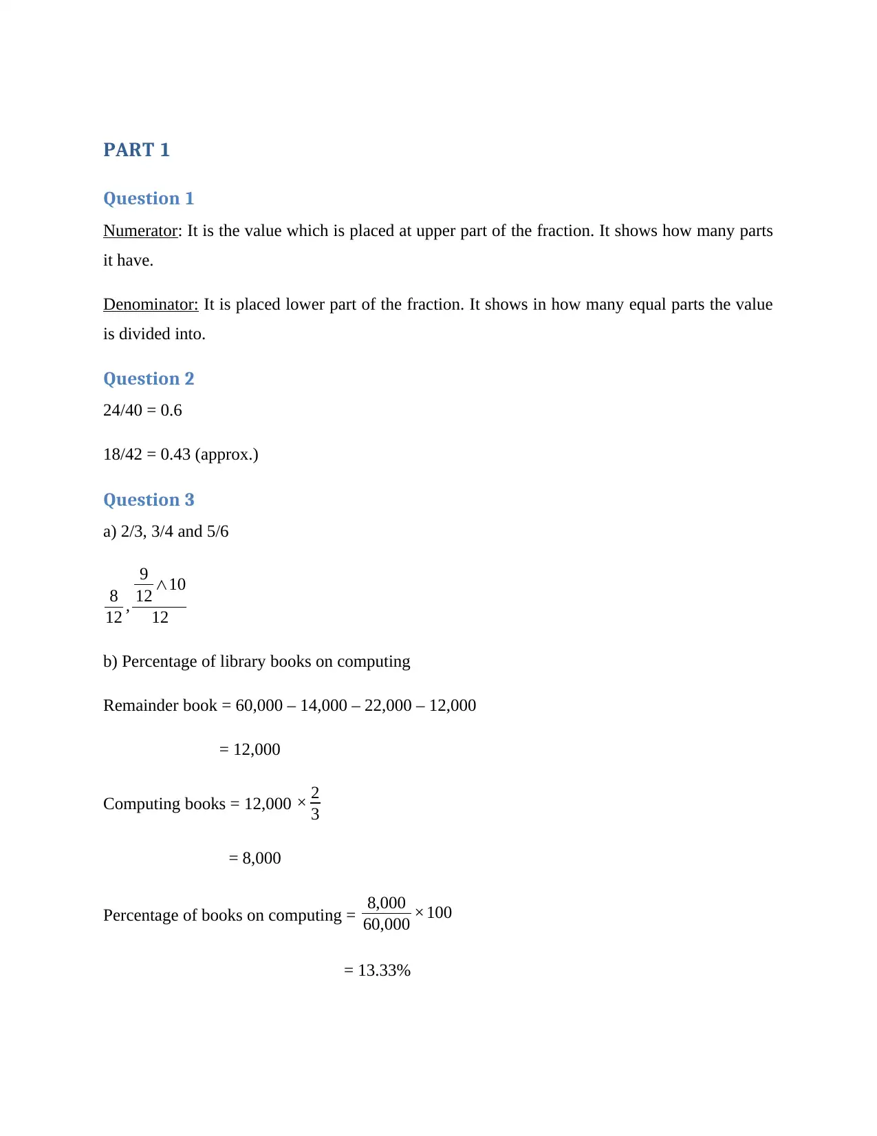
PART 1
Question 1
Numerator: It is the value which is placed at upper part of the fraction. It shows how many parts
it have.
Denominator: It is placed lower part of the fraction. It shows in how many equal parts the value
is divided into.
Question 2
24/40 = 0.6
18/42 = 0.43 (approx.)
Question 3
a) 2/3, 3/4 and 5/6
8
12 ,
9
12 ∧10
12
b) Percentage of library books on computing
Remainder book = 60,000 – 14,000 – 22,000 – 12,000
= 12,000
Computing books = 12,000 × 2
3
= 8,000
Percentage of books on computing = 8,000
60,000 ×100
= 13.33%

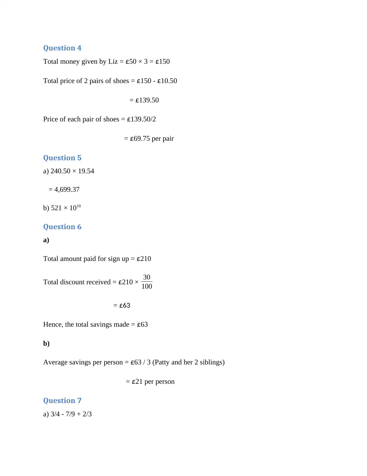
Question 4
Total money given by Liz = £50 × 3 = £150
Total price of 2 pairs of shoes = £150 - £10.50
= £139.50
Price of each pair of shoes = £139.50/2
= £69.75 per pair
Question 5
a) 240.50 × 19.54
= 4,699.37
b) 521 × 1010
Question 6
a)
Total amount paid for sign up = £210
Total discount received = £210 × 30
100
= £63
Hence, the total savings made = £63
b)
Average savings per person = £63 / 3 (Patty and her 2 siblings)
= £21 per person
Question 7
a) 3/4 - 7/9 + 2/3

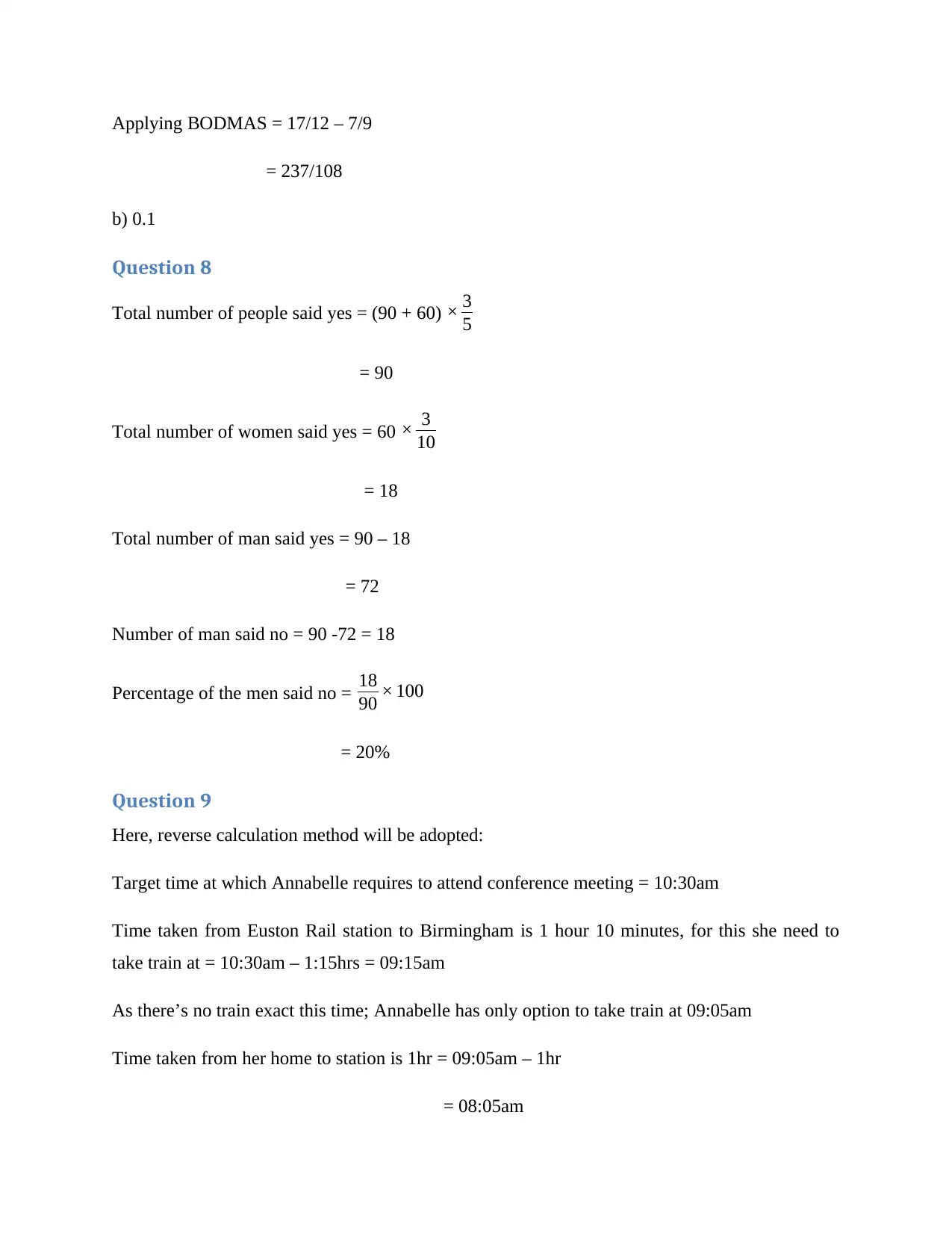
Applying BODMAS = 17/12 – 7/9
= 237/108
b) 0.1
Question 8
Total number of people said yes = (90 + 60) × 3
5
= 90
Total number of women said yes = 60 × 3
10
= 18
Total number of man said yes = 90 – 18
= 72
Number of man said no = 90 -72 = 18
Percentage of the men said no = 18
90 × 100
= 20%
Question 9
Here, reverse calculation method will be adopted:
Target time at which Annabelle requires to attend conference meeting = 10:30am
Time taken from Euston Rail station to Birmingham is 1 hour 10 minutes, for this she need to
take train at = 10:30am – 1:15hrs = 09:15am
As there’s no train exact this time; Annabelle has only option to take train at 09:05am
Time taken from her home to station is 1hr = 09:05am – 1hr
= 08:05am

Therefore; she needs to leave home at 08:05am.
Question 10
Converting both values in simple form = 9/25
= 0.36Kg
Therefore, 0.36 Kg or 9/25 Kg is heavier than 0.35Kg of Shredded Wheat.
Part 2
11)
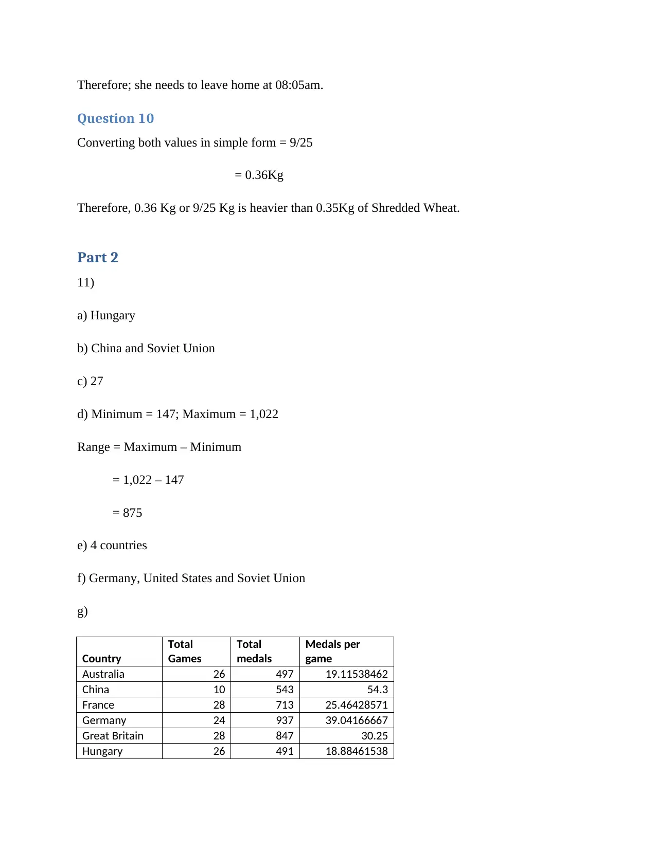
a) Hungary
b) China and Soviet Union
c) 27
d) Minimum = 147; Maximum = 1,022
Range = Maximum – Minimum
= 1,022 – 147
= 875
e) 4 countries
f) Germany, United States and Soviet Union
g)
Country
Total
Games
Total
medals
Medals per
game
Australia 26 497 19.11538462
China 10 543 54.3
France 28 713 25.46428571
Germany 24 937 39.04166667
Great Britain 28 847 30.25
Hungary 26 491 18.88461538

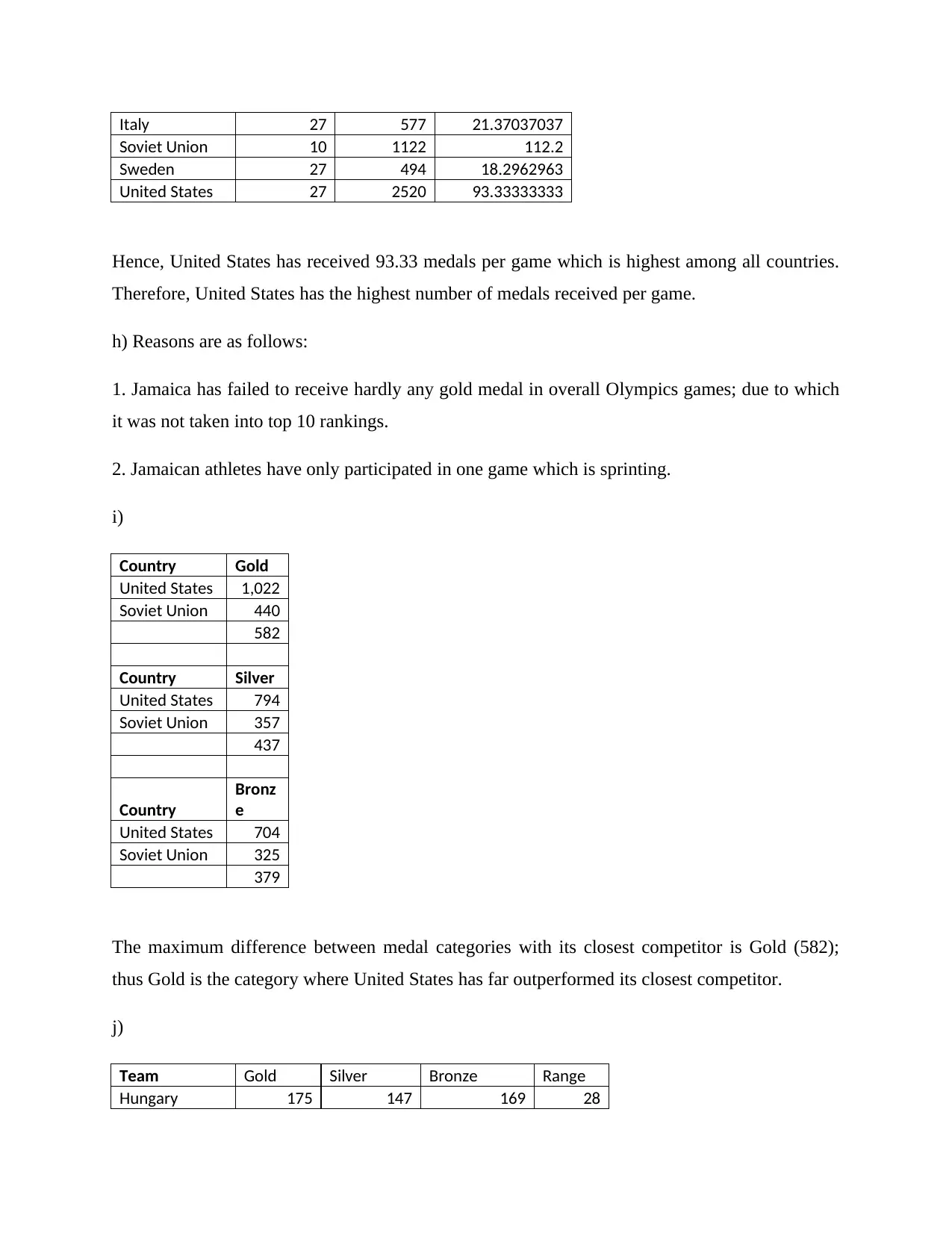
Italy 27 577 21.37037037
Soviet Union 10 1122 112.2
Sweden 27 494 18.2962963
United States 27 2520 93.33333333
Hence, United States has received 93.33 medals per game which is highest among all countries.
Therefore, United States has the highest number of medals received per game.
h) Reasons are as follows:
1. Jamaica has failed to receive hardly any gold medal in overall Olympics games; due to which
it was not taken into top 10 rankings.
2. Jamaican athletes have only participated in one game which is sprinting.
i)
Country Gold
United States 1,022
Soviet Union 440
582
Country Silver
United States 794
Soviet Union 357
437
Country
Bronz
e
United States 704
Soviet Union 325
379
The maximum difference between medal categories with its closest competitor is Gold (582);
thus Gold is the category where United States has far outperformed its closest competitor.
j)
Team Gold Silver Bronze Range
Hungary 175 147 169 28

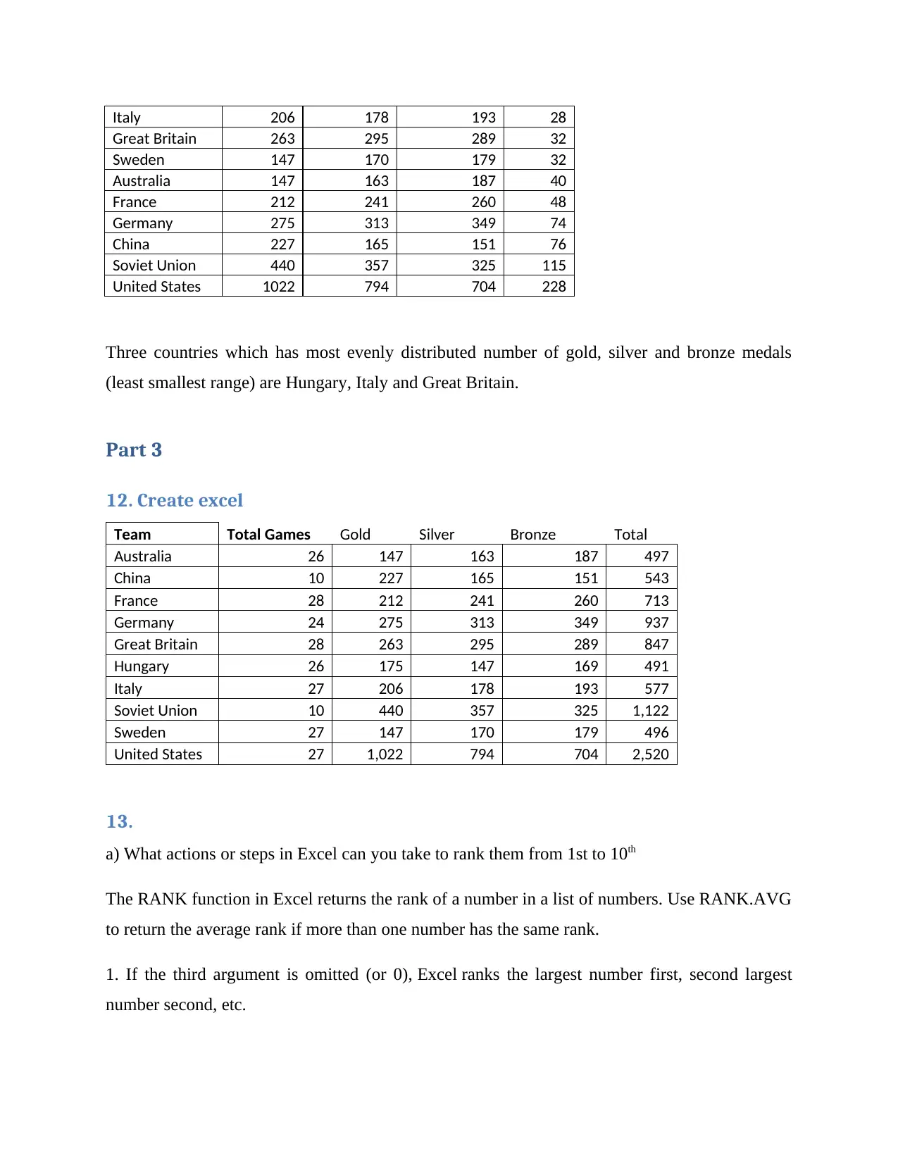
Italy 206 178 193 28
Great Britain 263 295 289 32
Sweden 147 170 179 32
Australia 147 163 187 40
France 212 241 260 48
Germany 275 313 349 74
China 227 165 151 76
Soviet Union 440 357 325 115
United States 1022 794 704 228
Three countries which has most evenly distributed number of gold, silver and bronze medals
(least smallest range) are Hungary, Italy and Great Britain.
Part 3
12. Create excel
Team Total Games Gold Silver Bronze Total
Australia 26 147 163 187 497
China 10 227 165 151 543
France 28 212 241 260 713
Germany 24 275 313 349 937
Great Britain 28 263 295 289 847
Hungary 26 175 147 169 491
Italy 27 206 178 193 577
Soviet Union 10 440 357 325 1,122
Sweden 27 147 170 179 496
United States 27 1,022 794 704 2,520
13.
a) What actions or steps in Excel can you take to rank them from 1st to 10th
The RANK function in Excel returns the rank of a number in a list of numbers. Use RANK.AVG
to return the average rank if more than one number has the same rank.
1. If the third argument is omitted (or 0), Excel ranks the largest number first, second largest
number second, etc.

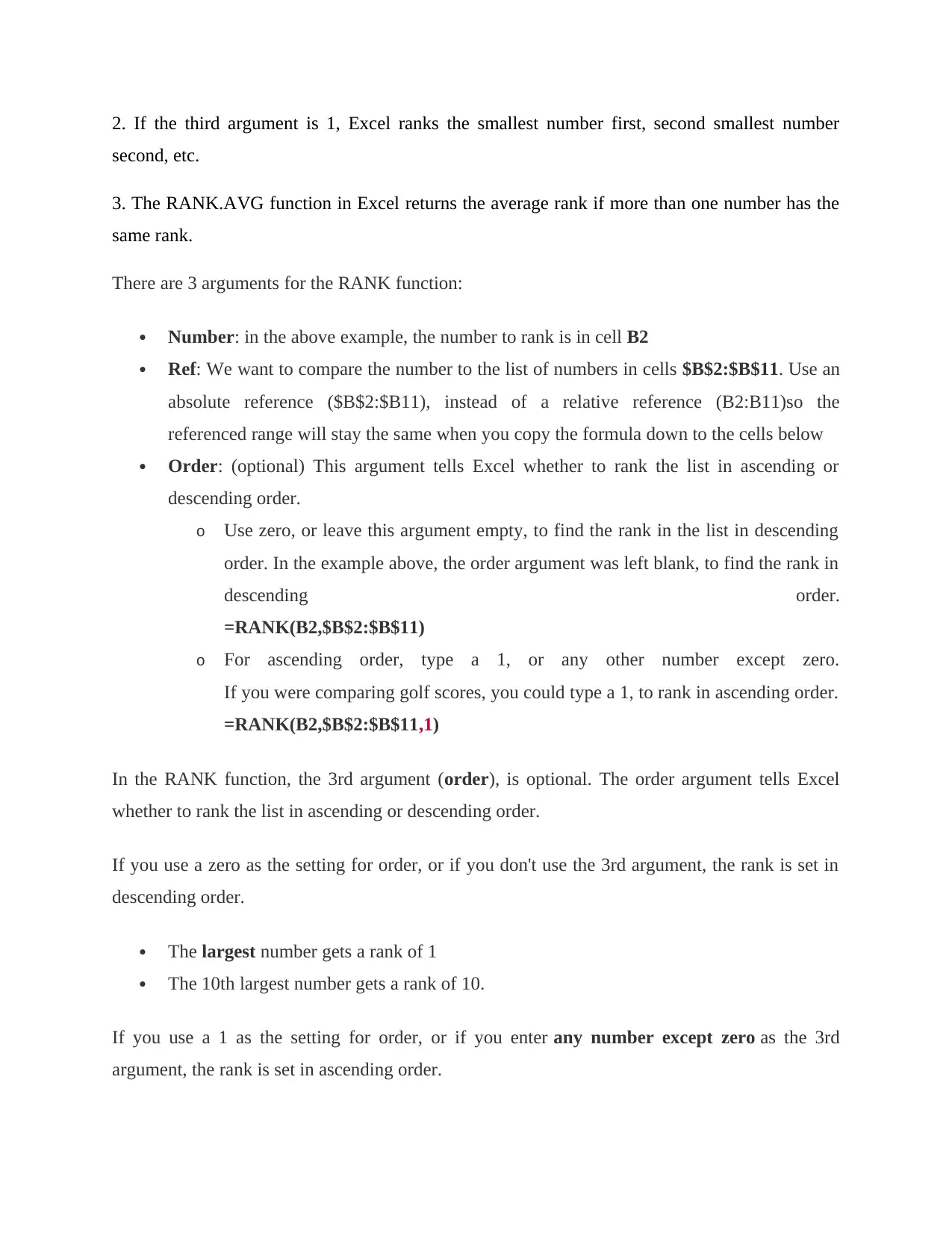
2. If the third argument is 1, Excel ranks the smallest number first, second smallest number
second, etc.
3. The RANK.AVG function in Excel returns the average rank if more than one number has the
same rank.
There are 3 arguments for the RANK function:
 Number: in the above example, the number to rank is in cell B2
 Ref: We want to compare the number to the list of numbers in cells $B$2:$B$11. Use an
absolute reference ($B$2:$B11), instead of a relative reference (B2:B11)so the
referenced range will stay the same when you copy the formula down to the cells below
 Order: (optional) This argument tells Excel whether to rank the list in ascending or
descending order.
o Use zero, or leave this argument empty, to find the rank in the list in descending
order. In the example above, the order argument was left blank, to find the rank in
descending order.
=RANK(B2,$B$2:$B$11)
o For ascending order, type a 1, or any other number except zero.
If you were comparing golf scores, you could type a 1, to rank in ascending order.
=RANK(B2,$B$2:$B$11,1)
In the RANK function, the 3rd argument (order), is optional. The order argument tells Excel
whether to rank the list in ascending or descending order.
If you use a zero as the setting for order, or if you don't use the 3rd argument, the rank is set in
descending order.
 The largest number gets a rank of 1
 The 10th largest number gets a rank of 10.
If you use a 1 as the setting for order, or if you enter any number except zero as the 3rd
argument, the rank is set in ascending order.

 The smallest number gets a rank of 1
 The 10th smallest number gets a rank of 10.
Instead of typing the order argument number into a RANK formula, use a cell reference, to
create a flexible formula.
For example, type a 1 in cell E1, and link to cell E1 for the order argument.
By linking to a cell, you can quickly see different results, without changing the formula. Type a
zero in cell E1, or delete the number, and the rank will change to Descending order.
For the order option, there are only 2 choices - Ascending or Descending. To make it easier for
people to change the order, use a check box to turning Ascending order ON or OFF.
 If it is turned ON, the RANK order will be Ascending
 If it is turned OFF, the RANK order will be Descending
b) State the specific action(s) or step(s) in Excel that will produce a list/display of those countries
with 800 or more medals in total?
To apply this action; conditional formatting is the excel tool which can visible the values below
800 through displaying it as different color. Below are the steps to get the result:
To build this basic formatting rule, follow these steps:
1. Select the information cells in the target field (cells C3: C14 in this template), click the Home
tab of the Excel ribbon, and then select Power Format ⇒ New Rule. The New Format Rule
Exchange box opens.
2. In the list box at the beginning of the switch box, click Use formula to find out which cells
make the selection. This decision assesses the values that depend on a particular recipe. On the

off chance that a particular value is not valued as TRUE, the restrictive group is deployed in that
cell.
3. In the recipe entry box, enter the equation shown here. Note that you can only refer to the
main cell in the target area. It is not necessary to mention the whole range.
4. Snap the Shape button. The Format Cells dialog box opens, where you have a full set of
alternatives to customize text style, margin, and fill for your target cell. After selecting your
organization options, click the "OK" button to confirm your progress and visit the New Format
Rule check box.
5. Again in the New Format Rule Talk box, click the "OK" button to confirm the group rule.
To show differential shading for cells below the measured value, the improvements are followed:
To compile this basic design guide, follow these methods: 1. Select the information cells in the
target area (cells E3: C14 in this form), click the Home tab of the Excel ribbon, then select New
Rule formatting of the finishing tool.
2. In the margin box at the top of the dialog box, click Use formula to determine in which cells to
choose a shape. This decision evaluates the values based on a specified equation. If a particular
value is evaluated TRUE, the restricted organization is deployed to that cell.
3. In the equation inbox, enter the recipe displayed with this progress. Note that you are basically
looking at your target cell (E3) with the stimulus in the test cell ($ B $ 3). As with normal
equations, you need to make sure that you use the references completely so that all stimuli in the
field are compared to the relevant correlation cell.

4. Snap the Shape button. This opens the Format Cells switchbox, where you have a full setup of
alternatives for the text style, margin, and fill for your target cell. When you're done selecting
your design options, click the OK button to confirm your progress and revisit the New Format
Rule Exchange box.
5. Again in the New Format Rule exchange box, click the OK button to confirm the design
principle.
c) Which type of graph will be suitable for representing only gold medals information?
Line graph or bar graph is more suitable in representing gold medal information
d) In which column(s) might replication have been used?
Total; in total column replicating formula of SUM for all other teams has been used.
e) What Excel formula can be used to calculate the overall total medals awarded?
=SUM() formula can be used to total overall medals
14) Write the Excel functions for the following
a. Give the total number of medals for Germany and Great Britain.
Formula:
= SUM(F32 + F38)
b. Give the average number of silver medals for a European country
Formula:
European countries = France, Germany, Great Britain, Italy, Soviet Union and Sweden
Total 6 counties.
=AVERAGE (F31 + F32 + F33 + F35 + F36 + F37)
c. Sum the Medals Total for Gold for those countries with less than 20 games involvement.