Numerical Analysis Assignment: Solution, Questions 1, 2, and 3

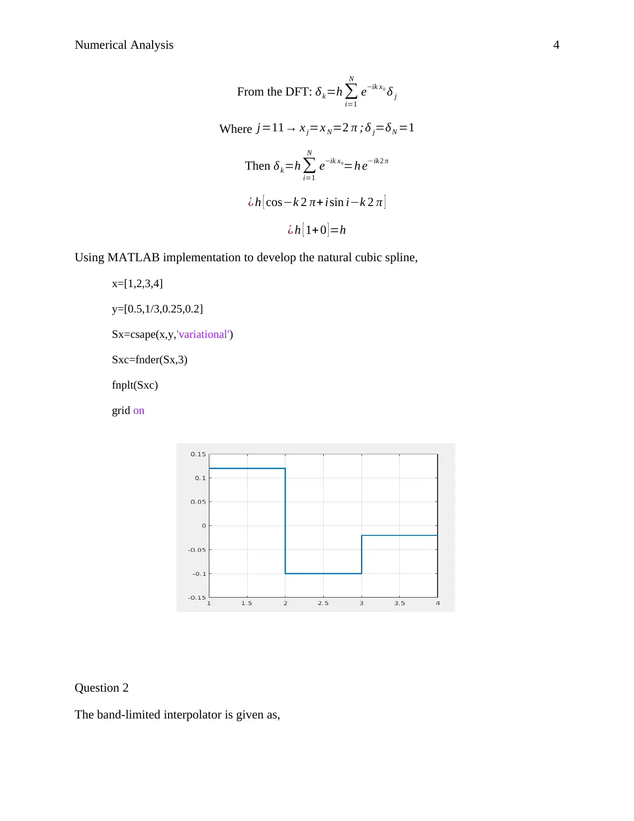
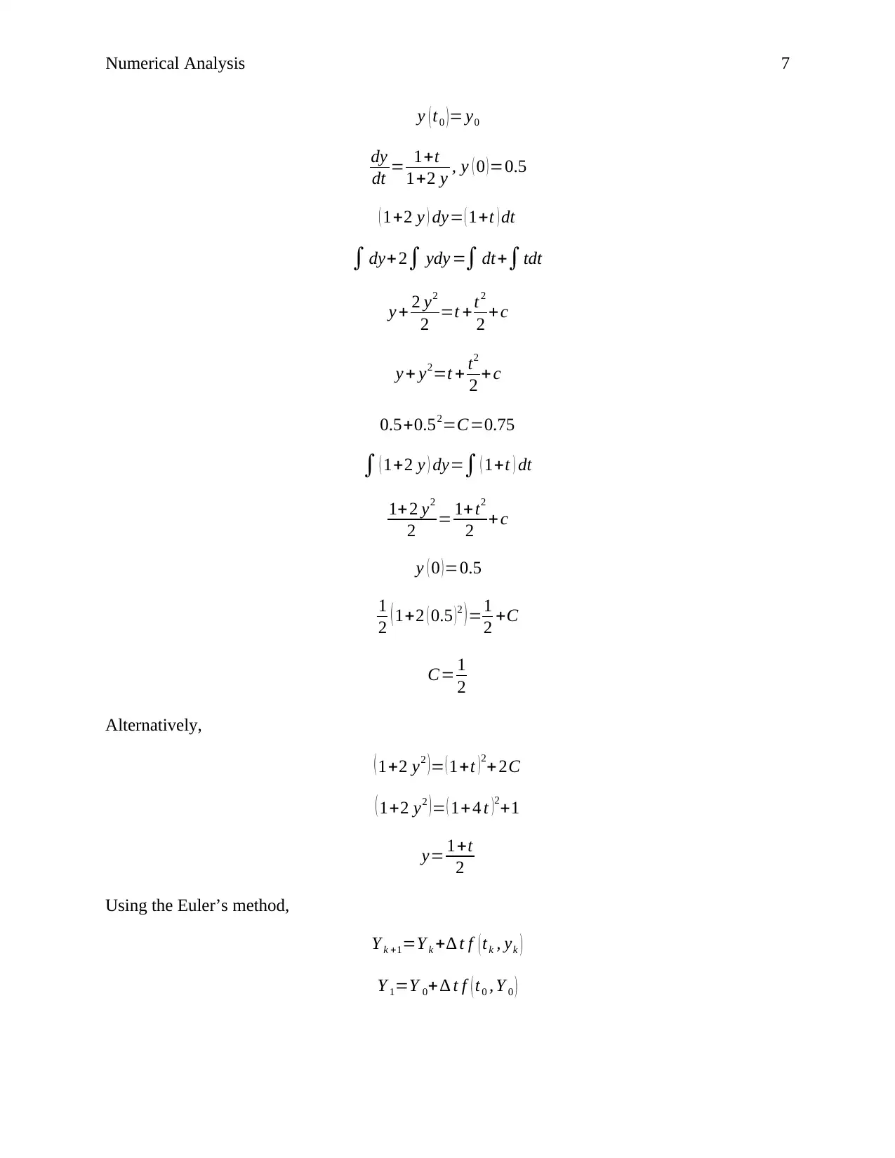
This document provides a comprehensive solution to a numerical analysis assignment. The solution covers three main questions. The first question involves data interpolation using a natural cubic spline, including the derivation of coefficients and the application of matrix methods for solving the spline's parameters. The second question addresses band-limited interpolation, detailing the derivation of the band-limited interpolator formula and its application. The third question focuses on numerical methods for solving ordinary differential equations (ODEs), specifically Euler's method, the midpoint method, and the fourth-order Runge-Kutta method, with detailed calculations and error analysis for each method.

Numerical Analysis 1
Numerical Analysis
Student Name
Student ID Number
Institutional Affiliation

Numerical Analysis 2
Question 1
The dataset is provided as,
Data item Value
1 (1,0.5)
2 (2,1/3)
3 (3,0.25)
4 (4,0.2)
The values are resolved such that the coefficients of the polynomials are,
a0=0. a1= 1
3 a2=0.25 a3=0.2
A⃗ z=⃗ u , Z0 =zn−natural cubic spline
A=
[ 1 0 0 0
h0 2 ( h0 +h1 ) h1 0
0 h1 2 ( h0+ h1 ) h2
0 0 0 1 ]
A=
[1 0 0 0
1 4 1 0
0 1 4 1
0 0 0 1 ]⃑
u=
[ 0
3
h1
(a2 −a1 ) − 3
h0
( a1 −a0 )
3
h2
(a3−a2 ) − 3
h1
( a2−a1 )
0
]=
0
0.25
0.1
0
A⃗ z=⃗ u
[1 0 0 0
1 4 1 0
0 1 4 1
0 0 0 1 ] [ z0
z1
z2
z3
]=
[ 0
0.25
0.1
0 ]
Solving further,

Numerical Analysis 3
z0=0
z0 +4 z1 + z2 + z3 =0.25
z1+ 4 z2 +z3=0.1
z3=0
s1 islinear∧S :(x:)= Z
S0 ( x )=0.5−0.18666 ( x−1 ) +0.02 ( x −1 )2
S0
' ( x )=−0.18666+ 0.06 ( x −1 )2
s0 (x)=0.12(1-1) = 0 = Z
S1 ( x ) =1
3 −0.12666 ( x −2 )+ 0.06 ( x−2 )2−0.01666 ( x−2 )3
S1
' ( x ) =−0.12666 ( x−2 ) +0.06 ( x−2 ) 2−0.0166 ( x −2 ) 2
S1 (x)=0.12 - 0.09996(x-2
S1 (x)= S1(2)=0.12
S2 ( x ) =0.25−0.05666 ( x −3 ) +0.01 ( x −3 )2−0.00333 ( x−3 )3
S2
' ( x ) =−0.05666+0.02 ( x−3 ) −0.00999 ( x−3 )2
S2 (x)=0.02-0.01998(x-3
S2 (x_2)=S_2 ( 3 )=0.02
S0 =a0 +b0 ( x−x0 ) +z0 ( x−x0 )2 +d0 ( x−x0 )3
S1=a1+b1 ( x−x1 ) + Z1 ( x−x1 )2 + d1 ( x−x2 )3
S2=a2 +b2 ( x−x2 ) + z2 ( x−x2 )2 +d2 ( x−x2 ) 3
Therefore,
si= { 1 i=N
0 otherwise }
Within the range of [0, 2π]

Numerical Analysis 4
From the DFT: δk=h ∑
i=1
N
e−ik x0
δ j
Where j=11→ x j=x N=2 π ; δ j=δN =1
Then δk=h ∑
i=1
N
e−ik x0
=h e−ik 2 π
¿ h [ cos−k 2 π+ isin i−k 2 π ]
¿ h [ 1+ 0 ] =h
Using MATLAB implementation to develop the natural cubic spline,
x=[1,2,3,4]
y=[0.5,1/3,0.25,0.2]
Sx=csape(x,y,'variational')
Sxc=fnder(Sx,3)
fnplt(Sxc)
grid on
Question 2
The band-limited interpolator is given as,

Numerical Analysis 5
P ( x ) = h
2 π ∑
k= N
2
Nx
3
e−ikx
¿ h
2 π
sin NX
2
tan X
2
=SN ( x )
The value is expressed further,
SN
' ( x )=
h
2 π [ tan x
2 cos Nx
2
N
2 −sin Nx
2 sec x
2
1
2 ]
tan x
2
¿ h
2 π [ N
2 cos Nx
2 cot x
2 = 1
2 sin ( Nx
2 ) csc2 x
2 ]
N
2 = π
h
Therefore,
¿ h
2 π [ π
h cos πx
h cot x
2 − 1
2 sin πx
h csc2 x
2 ]
¿ h
2 π [ π
h cos πjh
h cot jh
2 ]
¿ h
2 π [ π
h cos jπ cot jh
2 ]
¿ 1
2 (−1 ) j cot ( jh
2 )
But,
1
h0
( a2−a0 )− h0
2 ( z1 +2 z0 )
¿ ( 1
3 −0.5 )−1
3 ( 0.06+0 )=−0.18666

Numerical Analysis 6
b1= 1
h1 ( a2−a1 ) − h1
3 ( z2 +2 z1 )
¿ ( 0.25− 1
3 ) −1
3 ( 0+2 ( 0.01 ) )
¿−0.05666
d0 = 1
3 h0
( z1−z0 )= 1
3 ( 0.06 )=0.02
d1= 1
3 h1
( z2−z1 )= 1
3 ( 0.01−0.06 )= 1
3 ( ¿ 0.05 )=−0.01666
d2= 1
3 h2
( z3−z2 ) =1
3 ( 0=0.01 ) = 1
3 ( −0.01 ) =−0.00333
S ( x ) =
{ 0.5−0.018666 ( x−1 ) +0.02 ( x−1 ) 3 xϵ [ 1,2 ]
1
3 −0.12666 ( x−2 ) +0.06 ( x−2 )2 −0.01666 ( x−2 ) 3 xϵ [ 2,3 ]
0.25−0.05666 ( x−3 ) + 0.0011 ( x−3 ) 2=0.00333 ( x−3 ) 3 xϵ [ 3,4 ] }
Solving further,
zi ( x−xi+1 )3
6 + Zi+1
6 h ( x− xi )3 + 1
h [f i +1−f i+ h2
6 ( zi −zi +1 ) ] ( x−xi ) +f i− h2
6 zi− 0.06
6 ( x−1 )3 + [ 1
3 −0.5+ 1
6 (−0.06 ) ( x−1 ) +0.5
¿ 0.5−0.17666 ( x−1 ) +0.01 ( x −1 ) 3
¿ 0.01 ( x−3 )3 + 0.01
6 ( x−2 )3 + [0.25− 1
3 + 1
6 ( 0.06−0.01 ) ] ( x−2 )+ 1
3 − 0.06
6
¿ 32333−0.075 ( x−2 ) + 0.001666 ( x −2 ) 3+ 0.01 ( x−3 ) 3
¿ 0,01 ( x−4 )3 +
[0.2−0.25+ 1
6 ( 0.01 ) ( x−3 ) +0.25− 0.01
6 ]
¿ 0.248−0.048333 ( x −3 ) +0.001666 ( x−4 ) 3
Question 3
¿ dy
dt =f ( t , y )

Numerical Analysis 7
y ( t0 )= y0
dy
dt = 1+t
1+2 y , y ( 0 ) =0.5
( 1+2 y ) dy= ( 1+t ) dt
∫ dy+ 2∫ ydy =∫ dt+∫tdt
y + 2 y2
2 =t + t2
2 + c
y + y2=t + t2
2 + c
0.5+0.52=C=0.75
∫ ( 1+2 y ) dy=∫ ( 1+t ) dt
1+2 y2
2 = 1+ t2
2 + c
y ( 0 )=0.5
1
2 ( 1+2 ( 0.5 ) 2 ) =1
2 +C
C= 1
2
Alternatively,
( 1+2 y2 )= ( 1+t )2+ 2C
( 1+2 y2 )= ( 1+4 t )2+1
y= 1+t
2
Using the Euler’s method,
Y k +1=Y k +∆ t f ( tk , yk )
Y 1=Y 0+ ∆ t f ( t0 , Y 0 )

Numerical Analysis 8
¿ 0.5+0.2 ( 1
2 ) =0.6
y1= (1+t
2 )t =0.6
=0.8
error =|Y 1− y1|=0.2
Using the Midpoint method,
Y k +1=Y k +∆ t f ( tk , yk )
Y k +1=Y k +∆ t f ( tk+ 1
2
, Y k+ 1
2 )
Y 1
2
=Y 0 + ∆ t
2 f ( t0 , Y 0 )
¿ 0.5+0.1 ( 1
2 )=0.55
Y 1=Y 0+ ∆ t f (t1
2
, y 1
2 )
¿ 0.5+0.2 f ( 0.55 , 0.55 )
¿ 0.647619
|Error=|Y 1− y1|=0.152381
Using the fourth runge kutta method,
Y k +1=Y k + 1
6 [ k1+ 2k 2+2 k3 +k4 ]
k1 =∆ t f ( t0 , y0 )
¿ 0.2 ( 1
1+2 ( 0.5 ) )=0.1
k 2=∆ t f (t 0 , y0 + k1
2 )
¿ 0.2 f (0 , 0.5 , 0.1
2 )

Numerical Analysis 9
¿−0.147615
k3 =∆ t f (t0 , y 0+ k 2
2 )
¿ 0.2∗1+ 0.55
1+ 2 ( 0.5738095 ) =0.1443458
K4 =∆ t f ( t 0 , y0 +k 3 )
¿ 0.2 1+0.6
1+2 ( 0.6443458 ) =0.1398178
Y 1=Y 0+ 1
6 ¿
¿ 0.5+0.13729=0.63729
error =|Y 1− y1|=0.16271