University ME108 Assignment 2: Engineering Analysis and Methods

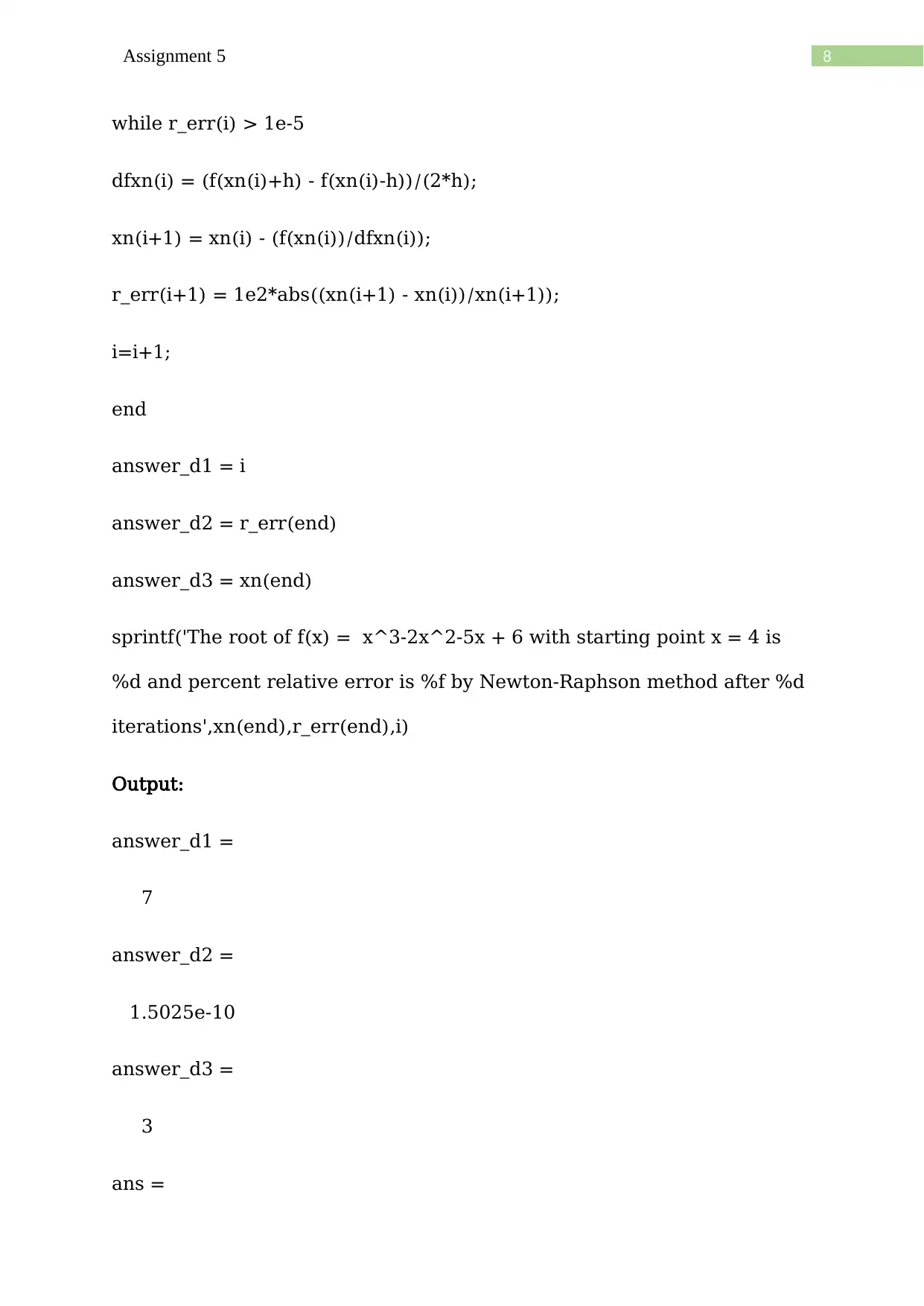
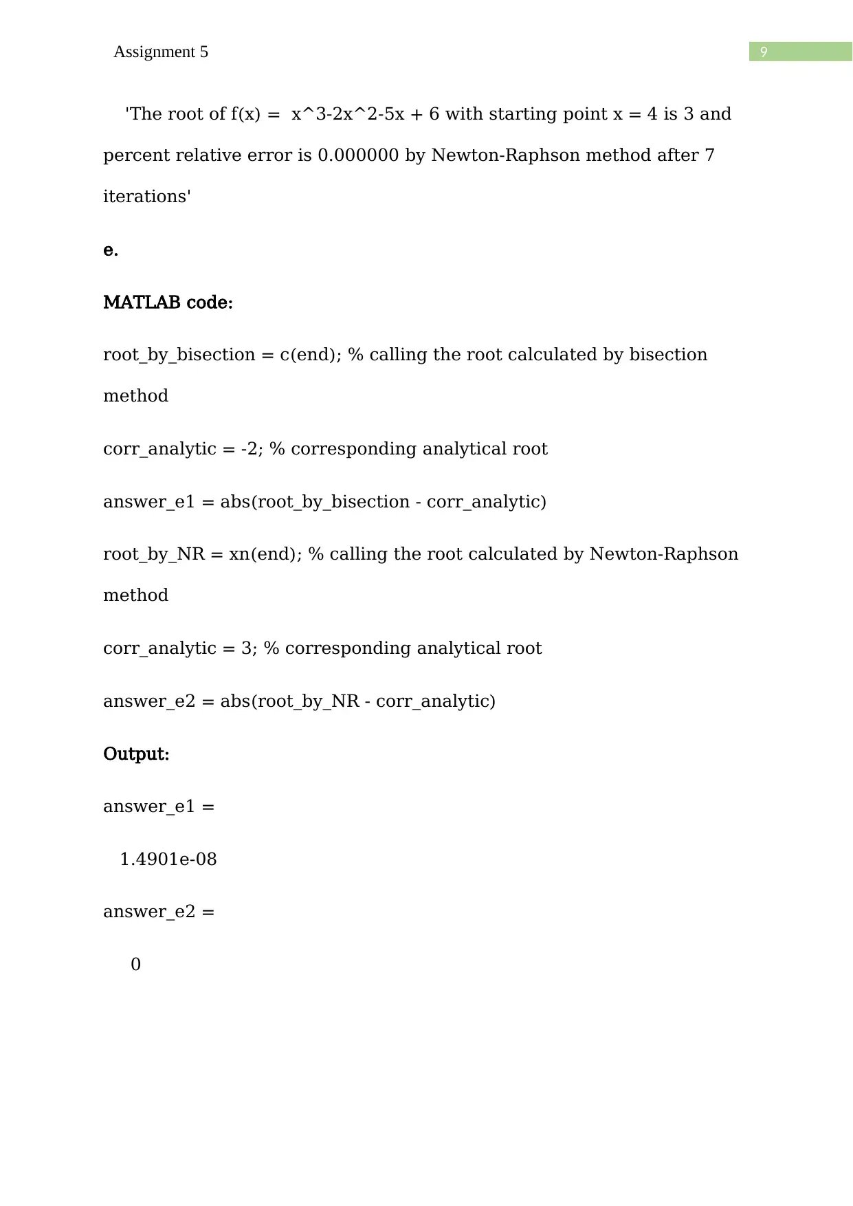
This document provides a comprehensive solution to ME108 Assignment 2, focusing on engineering analysis and numerical methods. The assignment involves finding roots of a cubic equation using analytical methods, Ruffini's rule, and graphical representation in MATLAB. The solution includes MATLAB code for each method, including the Bisection method and Newton-Raphson method, with detailed explanations, outputs, and analysis of relative errors. The document also compares the results obtained from different methods and discusses their accuracy. The assignment brief is also included, outlining the requirements and submission guidelines. The solution is designed to help students understand and apply numerical methods to solve engineering problems.

Running head: ASSIGNMENT 2
ME108 ENGINEERING ANALYSIS AND NUMERICAL METHODS
ASSIGNMENT 2
Name of the Student
Name of the University
Author Note

1Assignment 5
a.
Given, the equation is,
y(x) = a3x^3 + a2x^2 + a1x + a0
The coefficients are
a3 = 1, a2 = -2, a1 = -5, a0 = 6.
Hence, the equation is
y ( x )=x3−2 x2−5 x +6
Now, an analytical method used to find one root of the equation. The initial point is taken as
0.
y(0) = 6. Hence x is increased by 1.
y(1) = 1 – 2 -5 +6 = 0.
Hence, one of the root of the equation is x = 1.
Hence, in factored form the expression of y(x) will be
y(x) = (x-1)(x^2 –x -6)
Now, the remaining roots i.e. the roots of x2 – x−6 are calculated by Ruffini's rule.
MATLAB code:
a3 = 1; a2 = -2; a1 = -5; a0 = 6; % defining the coeffcient
f = @(x)(a3*x^3 + a2*x^2 +a1*x + a0);
x0 = 0;
while f(x0) ~= 0

2Assignment 5
x0 = x0 + 1;
end
answer_a1 = x0
sprintf('the analytical root is %d',answer_a1)
b1 = 1; b2 = -1; b3 = -6;
rufmat = [b1 b2 b3;0 0 0]; % the Ruffini's table
root2 = 1; % initial leftmost multiplier
rightmostval = (b1*root2 + b2)*root2 + b3; % calculation of right most value in Ruffini table
% Ruffini's method for finding the positive root
while rightmostval ~= 0
root2 = root2 + 1;
rightmostval = (b1*root2 + b2)*root2 + b3;
end
answer_a2 = root2
sprintf('the positive root by Ruffini method is %d',answer_a2)
% Ruffini's method for finding the negative root
root3 = -1; % initial leftmost multiplier

3Assignment 5
rightmostval = (b1*root3 + b2)*root3 + b3;
while rightmostval ~= 0
root3 = root3 - 1;
rightmostval = (b1*root3 + b2)*root3 + b3;
end
answer_a3 = root3
sprintf('the negative root by Ruffini method is %d',answer_a3)
Output:
answer_a1 =
1
ans =
'the analytical root is 1'
answer_a2 =
3
ans =
'the positive root by Ruffini method is 3'
answer_a3 =
-2

4Assignment 5
ans =
'the negative root by Ruffini method is -2'
b.
MATLAB code:
a3 = 1; a2 = -2; a1 = -5; a0 = 6;
x = -4:0.1:5;
f = a3.*(x.^3) + a2.*(x.^2) +a1.*x + a0;
plot(x,f,'b*')
grid on
hold on
plot(-2,0,'ro','linewidth',2);plot(1,0,'ro','linewidth',2);plot(3,0,'ro','linewidth',2)
title('y = f(x)')
xlabel('x values in range [-4,5]')
ylabel('y values correponding to x')
Output:

5Assignment 5
-4 -3 -2 -1 0 1 2 3 4 5
x values in range [-4,5]
-80
-60
-40
-20
0
20
40
60
y values correponding to x
y = f(x)
c.
a3 = 1; a2 = -2; a1 = -5; a0 = 6;
f = @(x)(a3*(x^3) + a2*(x^2) +a1*(x) + a0);
a = -4; % f(a)<0
b = 5; % f(b)> 0
% bisection method
c(1) = (a+b)/2;
if f(c(1)) > 0
b=c(1);
c(2) = (a+b)/2;

6Assignment 5
elseif f(c(1))< 0
a = c(1);
c(2) = (a+b)/2;
end
r_err(1) = 1e2*abs((c(2) - c(1))/c(2));i=1;
while r_err(i) > 1e-5 % applying relative error condition
if f(c(i)) > 0
b=c(i);
c(i+1) = (a+b)/2;
elseif f(c(i))< 0
a = c(i);
c(i+1) = (a+b)/2;
end
r_err(i+1) = 1e2*abs((c(i+1) - c(i))/c(i+1));
i=i+1;
end
sprintf('The root of f(x) = x^3-2x^2-5x + 6 in the domain [-4,5] is %f and percent relative
error is %f by bisection method after %d iterations',c(end),r_err(end),i)
answer_c1 = i-1
answer_c2 = r_err(end)

7Assignment 5
answer_c3 = c(end)
Output:
ans =
'The root of f(x) = x^3-2x^2-5x + 6 in the domain [-4,5] is -2.000000 and percent relative
error is 0.000007 by bisection method after 26 iterations'
answer_c1 =
25
answer_c2 =
6.7055e-06
answer_c3 =
-2.0000
d.
a3 = 1; a2 = -2; a1 = -5; a0 = 6; % defining the coeffcients
f = @(x)(a3*x^3 + a2*x^2 +a1*x + a0);
h = 1e-10; % specifying very small h in limit theorem
xn(1) = 4; % initial value
dfxn(1) = (f(xn(1)+h) - f(xn(1)-h))/(2*h); % calculating derivative at x1=
4 by limit theorem of derivative
xn(2) = xn(1) - (f(xn(1))/dfxn(1)); % Newton-Raphson iteration
r_err(1) = 1e2*abs((xn(2) - xn(1))/xn(2));i=1;

8Assignment 5
while r_err(i) > 1e-5
dfxn(i) = (f(xn(i)+h) - f(xn(i)-h))/(2*h);
xn(i+1) = xn(i) - (f(xn(i))/dfxn(i));
r_err(i+1) = 1e2*abs((xn(i+1) - xn(i))/xn(i+1));
i=i+1;
end
answer_d1 = i
answer_d2 = r_err(end)
answer_d3 = xn(end)
sprintf('The root of f(x) = x^3-2x^2-5x + 6 with starting point x = 4 is
%d and percent relative error is %f by Newton-Raphson method after %d
iterations',xn(end),r_err(end),i)
Output:
answer_d1 =
7
answer_d2 =
1.5025e-10
answer_d3 =
3
ans =

9Assignment 5
'The root of f(x) = x^3-2x^2-5x + 6 with starting point x = 4 is 3 and
percent relative error is 0.000000 by Newton-Raphson method after 7
iterations'
e.
MATLAB code:
root_by_bisection = c(end); % calling the root calculated by bisection
method
corr_analytic = -2; % corresponding analytical root
answer_e1 = abs(root_by_bisection - corr_analytic)
root_by_NR = xn(end); % calling the root calculated by Newton-Raphson
method
corr_analytic = 3; % corresponding analytical root
answer_e2 = abs(root_by_NR - corr_analytic)
Output:
answer_e1 =
1.4901e-08
answer_e2 =
0

10Assignment 5