Applied Numerical Methods Project 1 & 2: Triple Pendulum and Beams

Verified

Added on  2023/04/20

|15
|1932
|266
Project
AI Summary
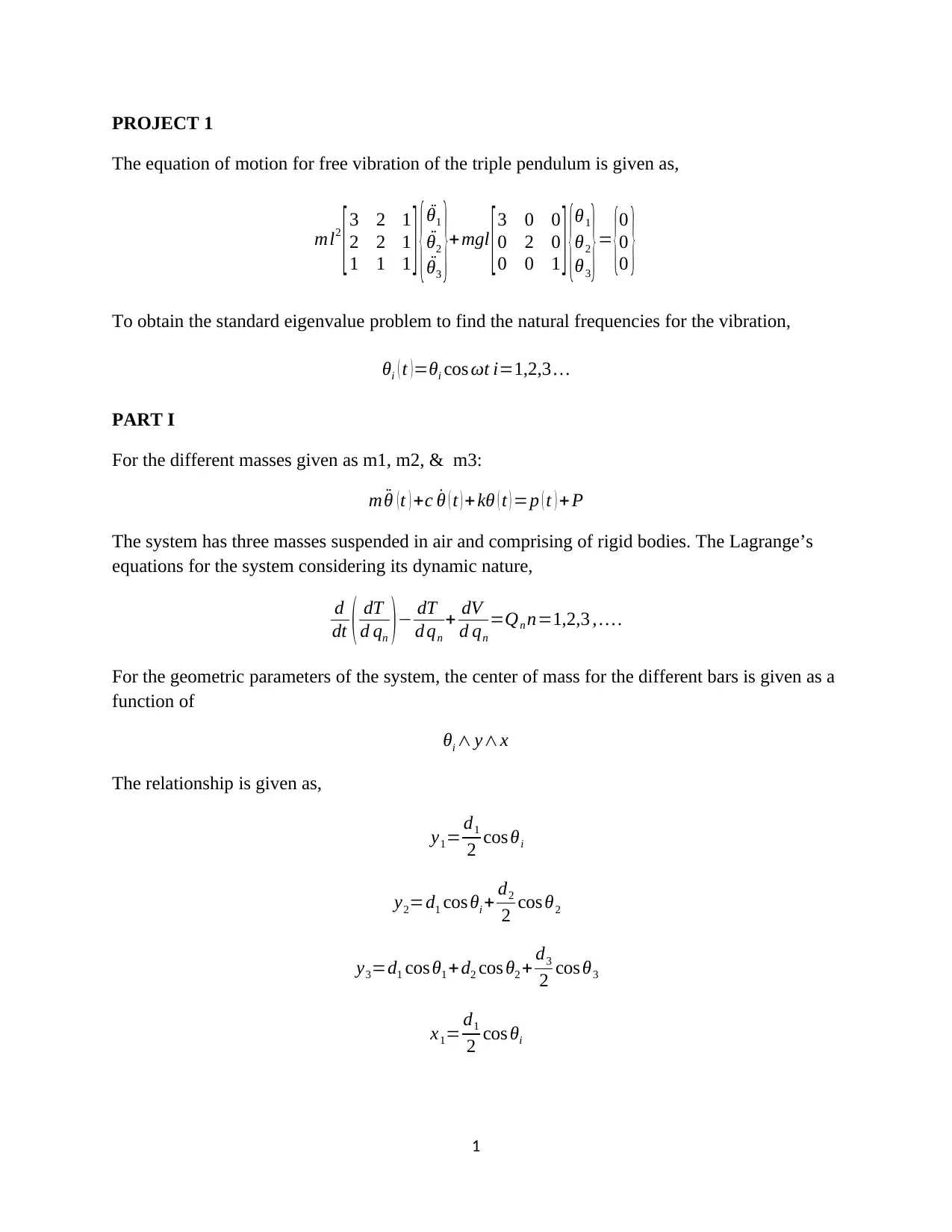
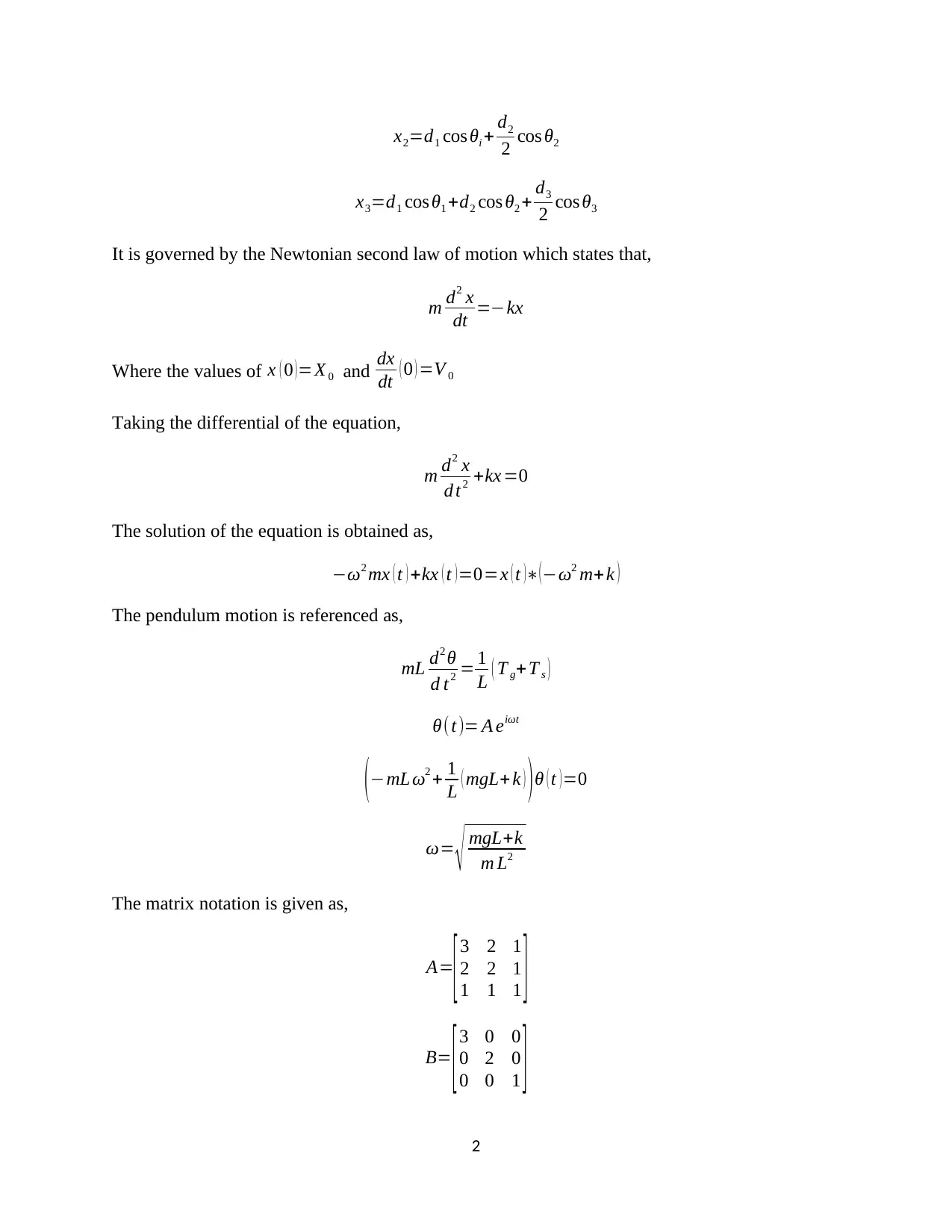
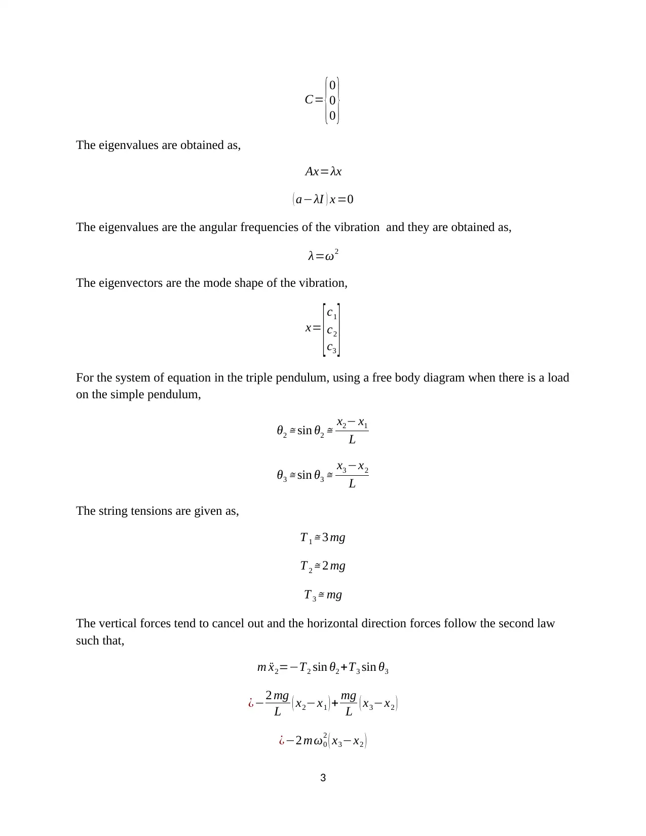
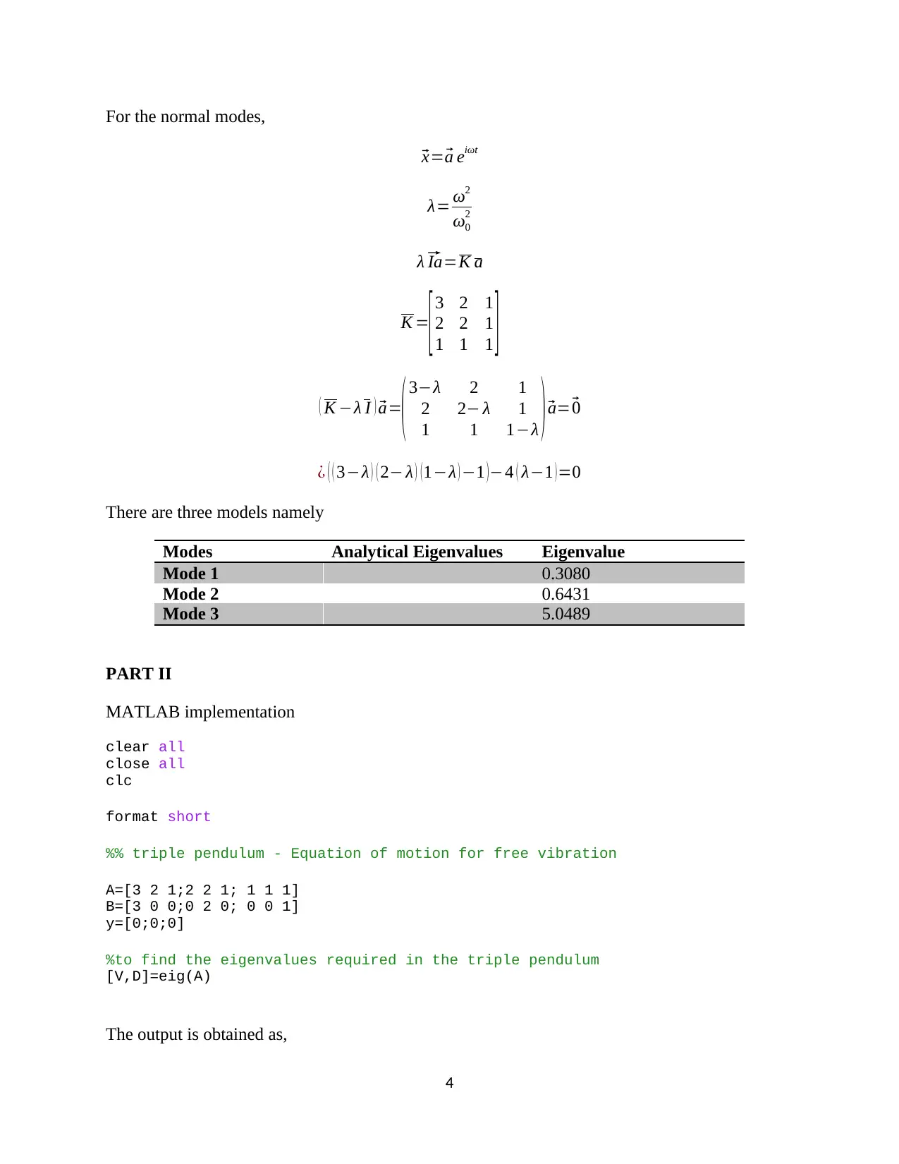
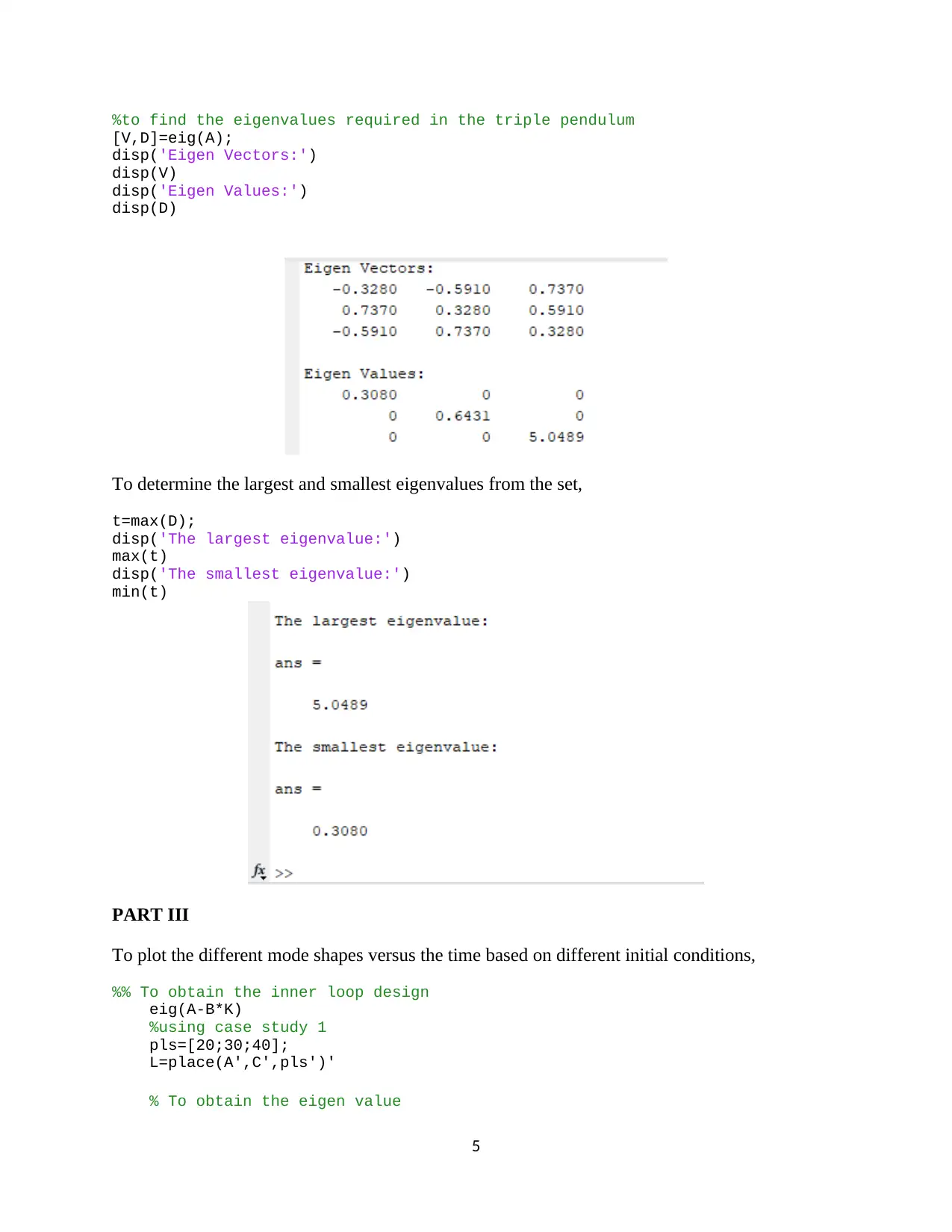
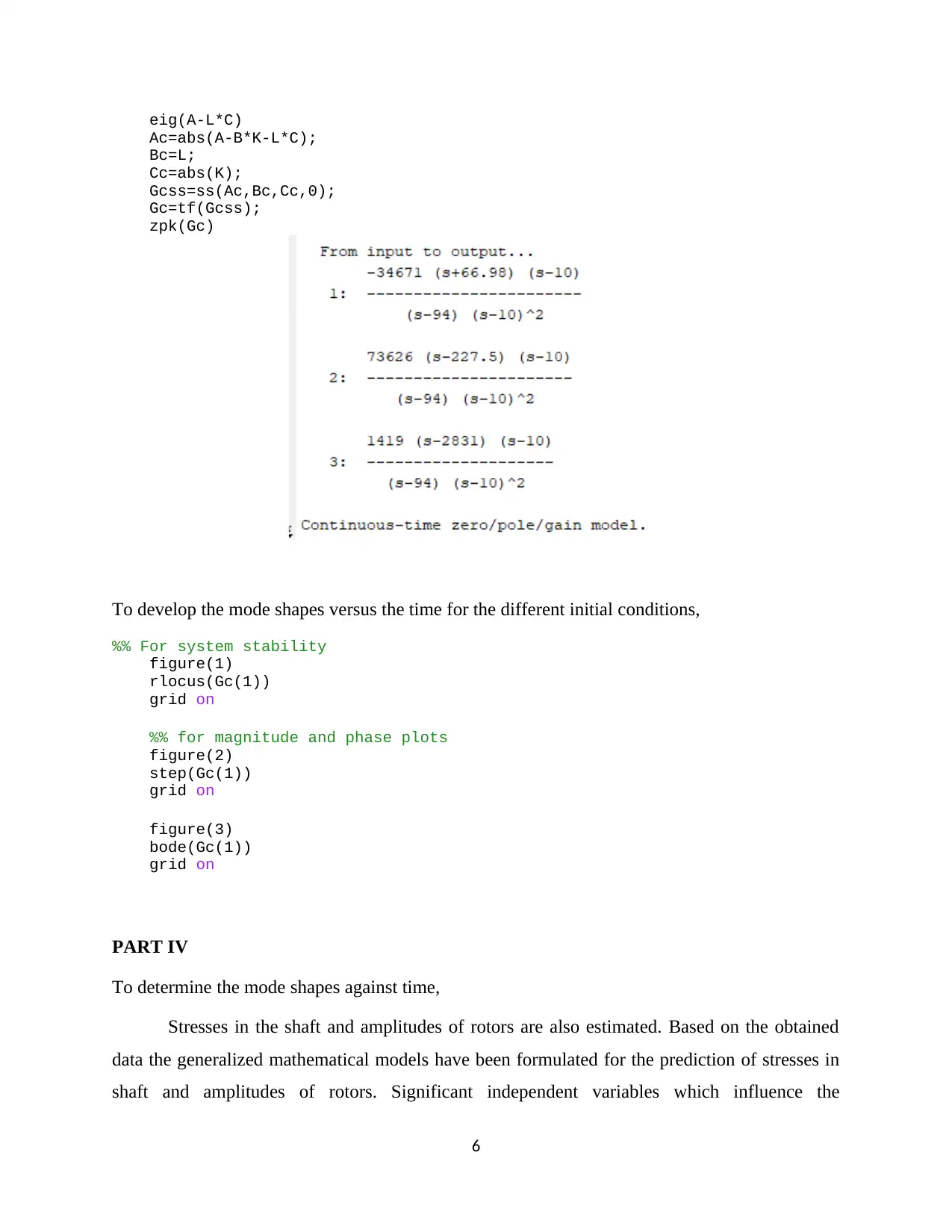
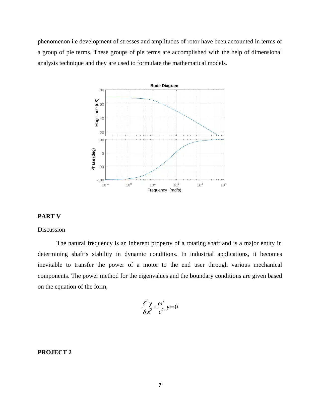
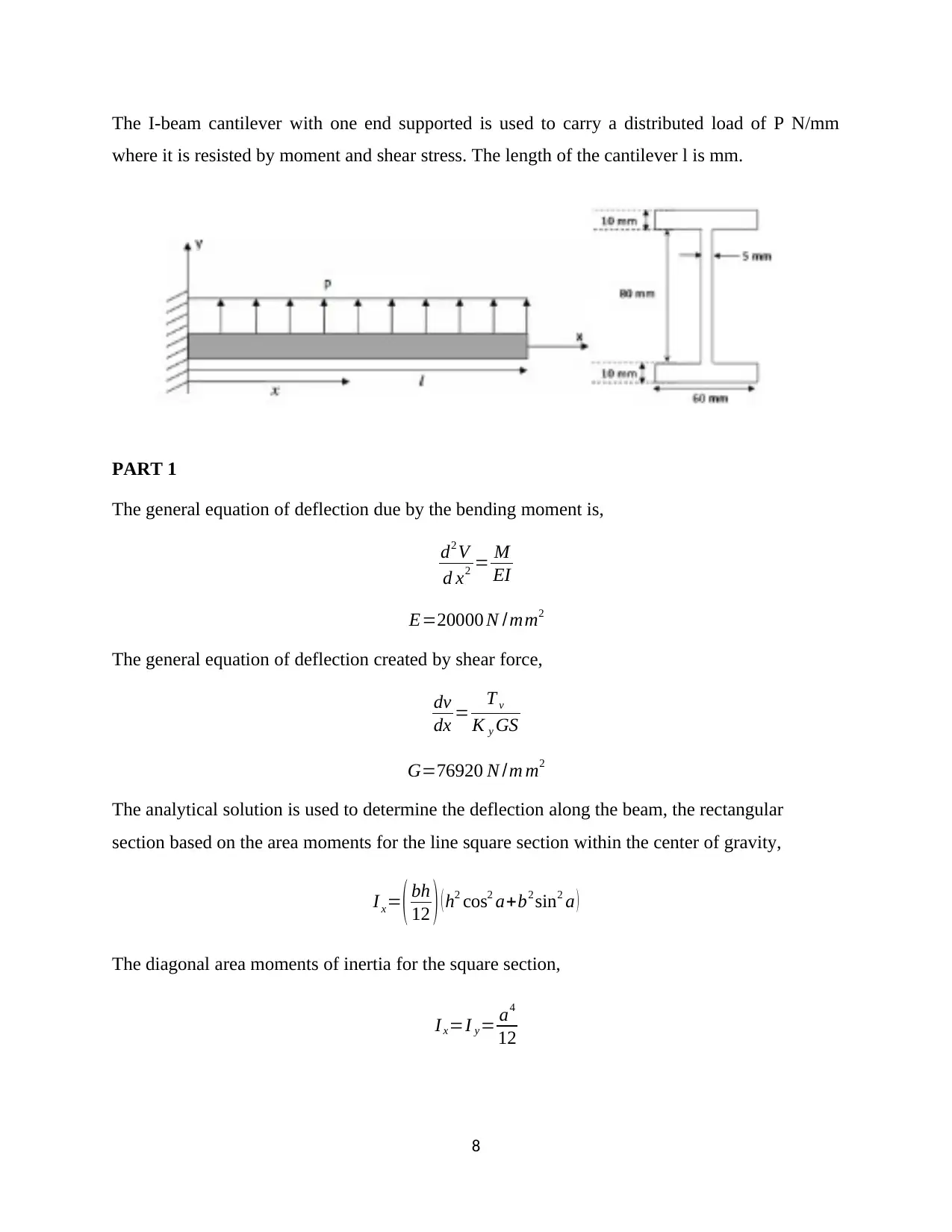
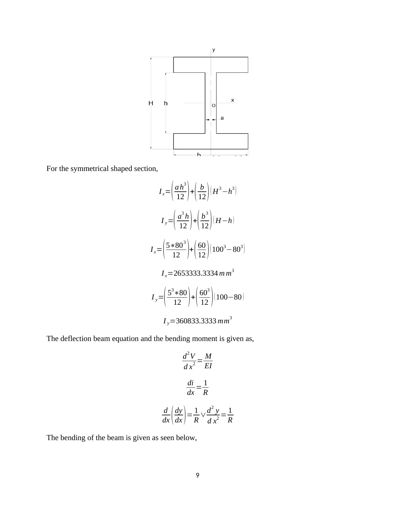
This project presents a comprehensive analysis of two mechanical engineering problems using applied numerical methods. Part I focuses on determining the natural frequencies of a triple pendulum's free vibration by formulating the equation of motion, deriving the eigenvalue problem, and obtaining analytical solutions. Part II involves implementing the problem in MATLAB to find eigenvalues and eigenvectors. Part III extends the MATLAB implementation to plot mode shapes versus time under various initial conditions, including system stability analysis, frequency response plots, and the design of an inner loop using control theory techniques such as the 'place' function and Bode diagrams. Part IV addresses the estimation of stresses in the shaft and rotor amplitudes. Part V provides a discussion on the natural frequency of a rotating shaft, including the power method for eigenvalues and boundary conditions. Project 2 focuses on the deflection analysis of an I-beam cantilever with a distributed load, utilizing analytical solutions for deflection and shear force calculations, and considering bending moments. Part II estimates deflection behavior using Runge-Kutta methods, and Part III provides a comparative discussion on the strength and deflection characteristics of T-beams, I-beams, and Z-beams, including strain diagram analysis and concluding that the I-beam is preferred for handling compressive and tensile pressures.
Document Page
SKMM3023 APPLIED
NUMERICAL METHODS
PROJECT 1 & 2
2018
tabler-icon-diamond-filled.svg

Paraphrase This Document

Need a fresh take? Get an instant paraphrase of this document with our AI Paraphraser
Document Page
PROJECT 1
The equation of motion for free vibration of the triple pendulum is given as,
ml2
[3 2 1
2 2 1
1 1 1 ] { ¨θ1
¨θ2
¨θ3
}+mgl [3 0 0
0 2 0
0 0 1 ] {θ1
θ2
θ3
}= {0
0
0 }
To obtain the standard eigenvalue problem to find the natural frequencies for the vibration,
θi ( t )=θi cos ωt i=1,2,3
PART I
For the different masses given as m1, m2, & m3:
m ¨θ (t ) +c ˙θ ( t ) + ( t ) =p ( t ) + P
The system has three masses suspended in air and comprising of rigid bodies. The Lagrange’s
equations for the system considering its dynamic nature,
d
dt ( dT
d qn ) dT
d qn
+ dV
d qn
=Qn n=1,2,3 , .
For the geometric parameters of the system, the center of mass for the different bars is given as a
function of
θi yx
The relationship is given as,
y1= d1
2 cos θi
y2=d1 cos θi + d2
2 cos θ2
y3=d1 cos θ1 + d2 cos θ2 + d3
2 cos θ3
x1= d1
2 cos θi
1
Document Page
x2=d1 cos θi + d2
2 cos θ2
x3=d1 cos θ1 +d2 cos θ2 + d3
2 cos θ3
It is governed by the Newtonian second law of motion which states that,
m d2 x
dt =kx
Where the values of x ( 0 ) =X 0 and dx
dt ( 0 ) =V 0
Taking the differential of the equation,
m d2 x
d t2 +kx =0
The solution of the equation is obtained as,
ω2 mx ( t ) +kx ( t ) =0=x ( t )( ω2 m+k )
The pendulum motion is referenced as,
mL d2 θ
d t2 = 1
L ( T g+T s )
θ(t)= A eiωt
(mL ω2 + 1
L ( mgL+ k ) )θ ( t )=0
ω= mgL+k
m L2
The matrix notation is given as,
A=
[3 2 1
2 2 1
1 1 1 ]
B= [3 0 0
0 2 0
0 0 1 ]
2
Document Page
C= {
0
0
0 }
The eigenvalues are obtained as,
Ax=λx
( aλI ) x =0
The eigenvalues are the angular frequencies of the vibration and they are obtained as,
λ=ω2
The eigenvectors are the mode shape of the vibration,
x=
[c1
c2
c3 ]
For the system of equation in the triple pendulum, using a free body diagram when there is a load
on the simple pendulum,
θ2 sin θ2 x2 x1
L
θ3 sin θ3 x3 x2
L
The string tensions are given as,
T 1 3 mg
T 2 2 mg
T 3 mg
The vertical forces tend to cancel out and the horizontal direction forces follow the second law
such that,
m ¨x2=T2 sin θ2 +T3 sin θ3
¿2 mg
L ( x2x1 ) + mg
L ( x3x2 )
¿2 mω0
2 ( x3x2 )
3
tabler-icon-diamond-filled.svg

Paraphrase This Document

Need a fresh take? Get an instant paraphrase of this document with our AI Paraphraser
Document Page
For the normal modes,
x= a eiωt
λ= ω2
ω0
2
λ Ia=K a
K =
[3 2 1
2 2 1
1 1 1 ]
( K λ I ) a=
(3λ 2 1
2 2 λ 1
1 1 1λ ) a= 0
¿ ( ( 3λ ) ( 2 λ ) (1λ ) 1 )4 ( λ1 )=0
There are three models namely
Modes Analytical Eigenvalues Eigenvalue
Mode 1 0.3080
Mode 2 0.6431
Mode 3 5.0489
PART II
MATLAB implementation
clear all
close all
clc
format short
%% triple pendulum - Equation of motion for free vibration
A=[3 2 1;2 2 1; 1 1 1]
B=[3 0 0;0 2 0; 0 0 1]
y=[0;0;0]
%to find the eigenvalues required in the triple pendulum
[V,D]=eig(A)
The output is obtained as,
4
Document Page
%to find the eigenvalues required in the triple pendulum
[V,D]=eig(A);
disp('Eigen Vectors:')
disp(V)
disp('Eigen Values:')
disp(D)
To determine the largest and smallest eigenvalues from the set,
t=max(D);
disp('The largest eigenvalue:')
max(t)
disp('The smallest eigenvalue:')
min(t)
PART III
To plot the different mode shapes versus the time based on different initial conditions,
%% To obtain the inner loop design
eig(A-B*K)
%using case study 1
pls=[20;30;40];
L=place(A',C',pls')'
% To obtain the eigen value
5
Document Page
eig(A-L*C)
Ac=abs(A-B*K-L*C);
Bc=L;
Cc=abs(K);
Gcss=ss(Ac,Bc,Cc,0);
Gc=tf(Gcss);
zpk(Gc)
To develop the mode shapes versus the time for the different initial conditions,
%% For system stability
figure(1)
rlocus(Gc(1))
grid on
%% for magnitude and phase plots
figure(2)
step(Gc(1))
grid on
figure(3)
bode(Gc(1))
grid on
PART IV
To determine the mode shapes against time,
Stresses in the shaft and amplitudes of rotors are also estimated. Based on the obtained
data the generalized mathematical models have been formulated for the prediction of stresses in
shaft and amplitudes of rotors. Significant independent variables which influence the
6
tabler-icon-diamond-filled.svg

Paraphrase This Document

Need a fresh take? Get an instant paraphrase of this document with our AI Paraphraser
Document Page
phenomenon i.e development of stresses and amplitudes of rotor have been accounted in terms of
a group of pie terms. These groups of pie terms are accomplished with the help of dimensional
analysis technique and they are used to formulate the mathematical models.
20
40
60
80
Magnitude (dB)
10-1 100 101 102 103 104
-180
-90
0
90
Phase (deg)
Bode Diagram
Frequency (rad/s)
PART V
Discussion
The natural frequency is an inherent property of a rotating shaft and is a major entity in
determining shaft’s stability in dynamic conditions. In industrial applications, it becomes
inevitable to transfer the power of a motor to the end user through various mechanical
components. The power method for the eigenvalues and the boundary conditions are given based
on the equation of the form,
δ2 y
δ x2 + ω2
c2 y=0
PROJECT 2
7
Document Page
The I-beam cantilever with one end supported is used to carry a distributed load of P N/mm
where it is resisted by moment and shear stress. The length of the cantilever l is mm.
PART 1
The general equation of deflection due by the bending moment is,
d2 V
d x2 = M
EI
E=20000 N /mm2
The general equation of deflection created by shear force,
dv
dx = T v
K y GS
G=76920 N /m m2
The analytical solution is used to determine the deflection along the beam, the rectangular
section based on the area moments for the line square section within the center of gravity,
I x= ( bh
12 ) ( h2 cos2 a+b2 sin2 a )
The diagonal area moments of inertia for the square section,
I x=I y= a4
12
8
Document Page
For the symmetrical shaped section,
I x= ( a h3
12 ) +( b
12 ) ( H3 h3 )
I y=( a3 h
12 ) +( b3
12 ) ( Hh )
I x= (5803
12 )+ ( 60
12 ) ( 1003803 )
I x=2653333.3334 m m3
I y=( 5380
12 ) + ( 603
12 ) ( 10080 )
I y=360833.3333 mm3
The deflection beam equation and the bending moment is given as,
d2 V
d x2 = M
EI
di
dx = 1
R
d
dx ( dy
dx ) = 1
R d2 y
d x2 = 1
R
The bending of the beam is given as seen below,
9
tabler-icon-diamond-filled.svg

Paraphrase This Document

Need a fresh take? Get an instant paraphrase of this document with our AI Paraphraser
Document Page
M =EI d2 y
d x2
To determine the shear force based on the rate of the intensity of loading as well as the shear
force,
dM
dx =EI d3 y
d x3
F=EI d3 y
d x3
PART 2
Estimating the deflection behavior along the beam using the approximation methods such as the
Runge Kutta midpoint or the Runge Kutta Ralston and RK4,
The general stress at each given point in the cantilever especially between each end and load,
s= W
2 Z ( 1
4 lx )
The deflection at any point is given as,
y= W x2
48 EI ( 3 l4 x )
There is a maximum deflection at a load, for the expression,
y= W l3
192 EI
yi+1 = yi+ d yi+1
dt h= yia yi+1 h
yi+1 = yi
1+ ah
Comparing the T-beam, I-beam, and z-beam,
load=repmat(10,1,1001);
l=20;
dl=0.02;
ei=1500; %Young Modulus
beam_deflection(load,ei,l,dl)
10
Document Page
11
chevron_up_icon
1 out of 15
circle_padding
hide_on_mobile
zoom_out_icon
[object Object]