Numerical Methods: Wave Equation Stability and Analysis Solution

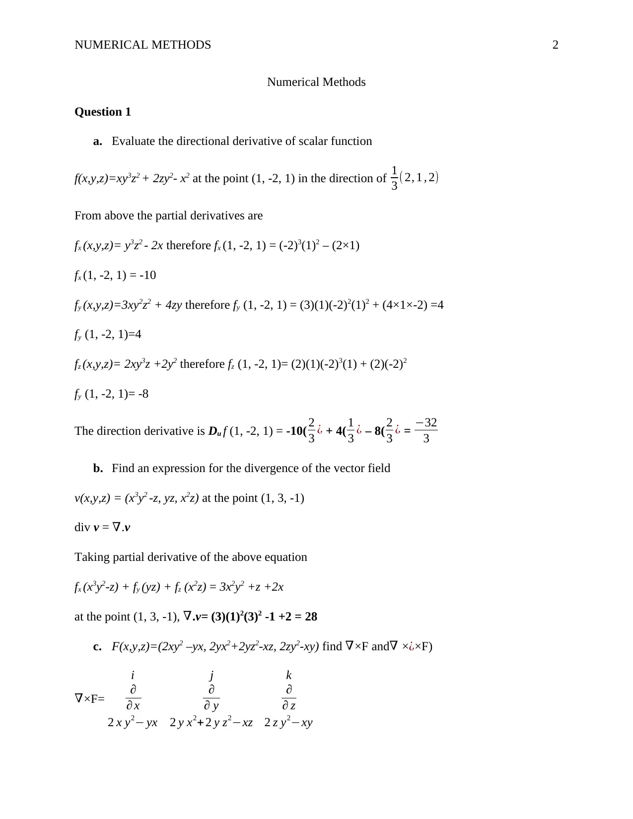
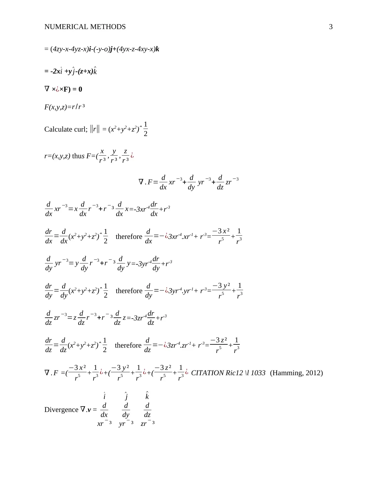
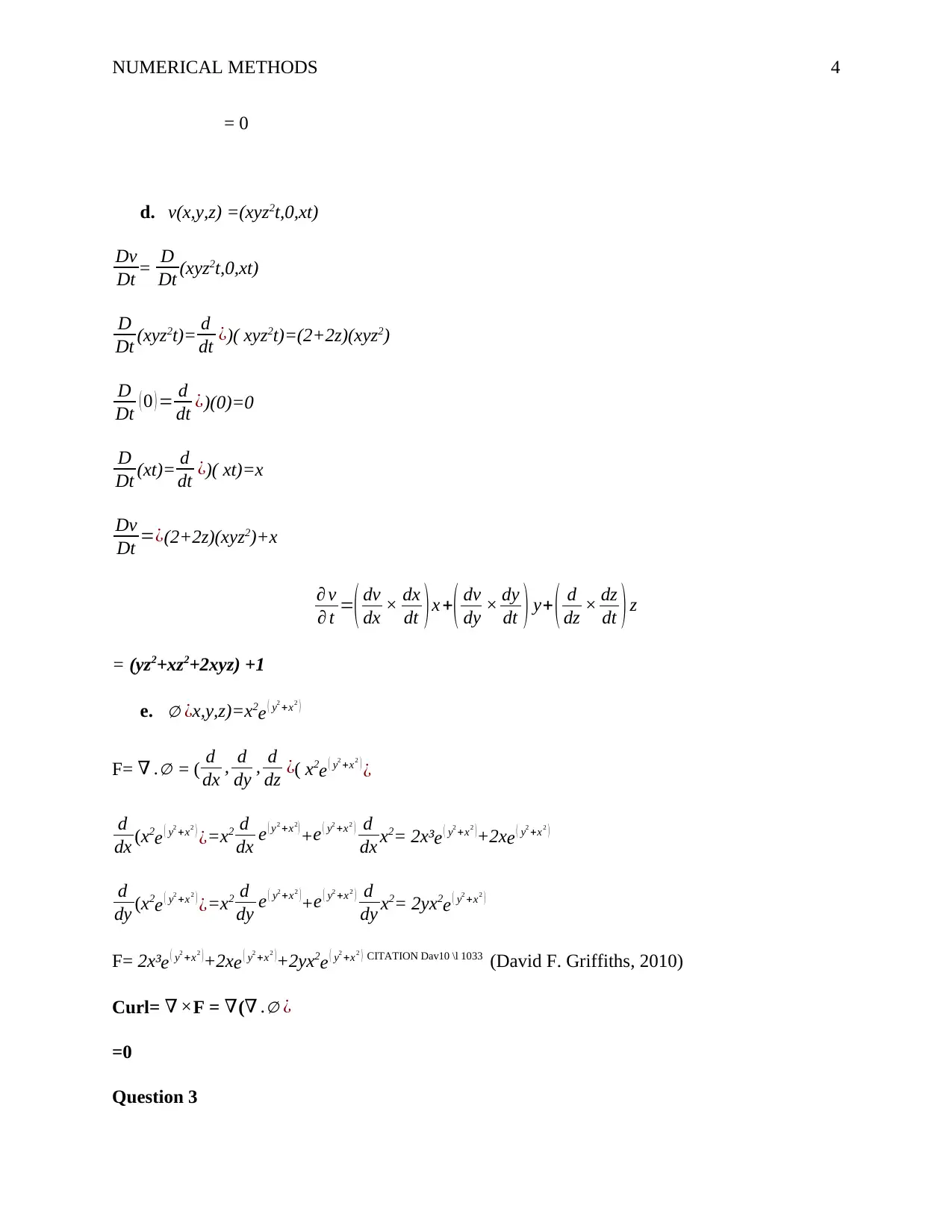
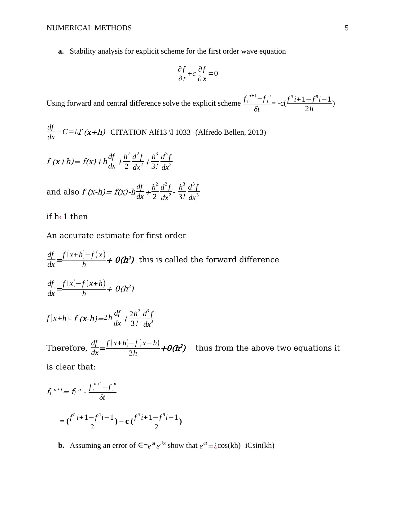
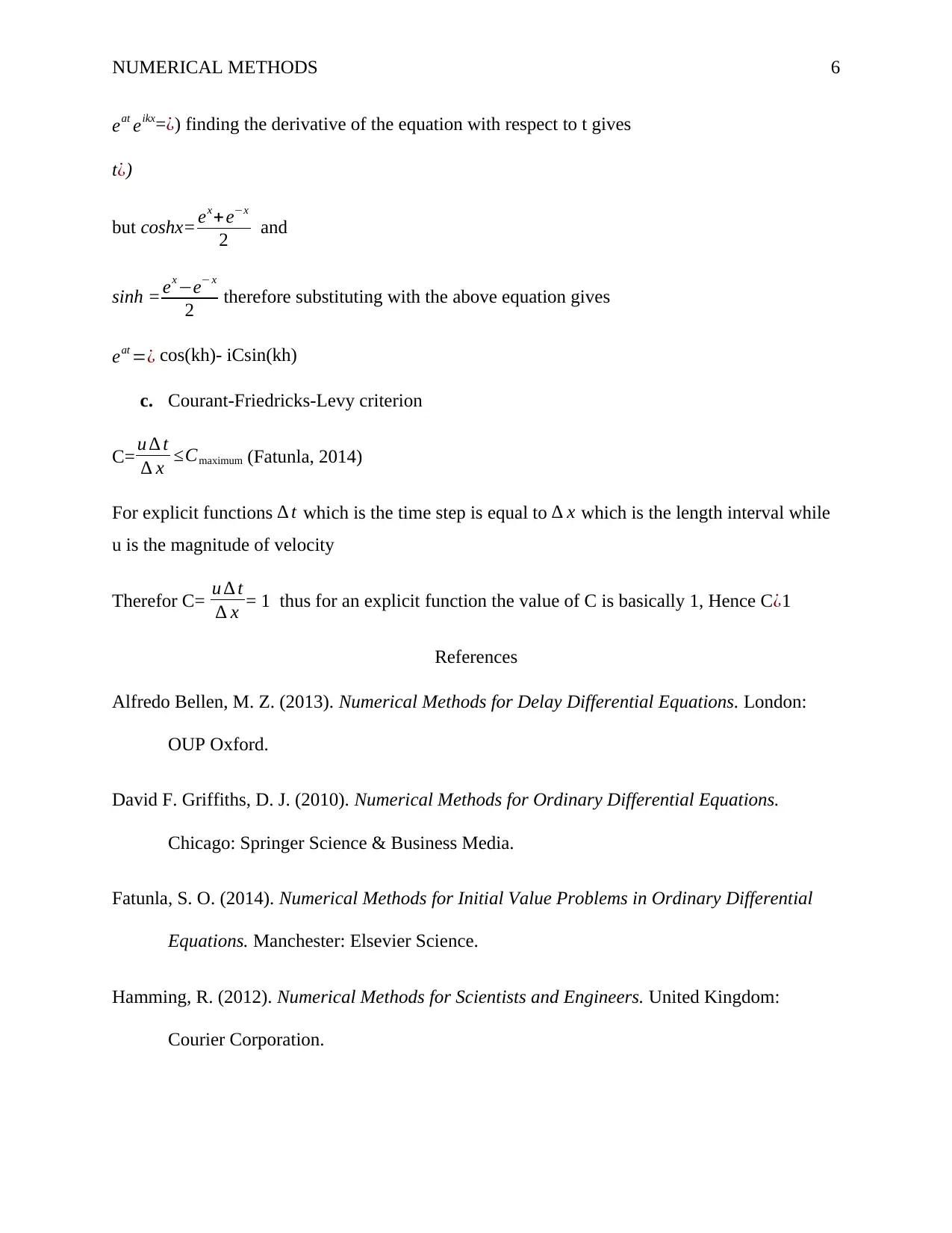
This assignment solution delves into various concepts within numerical methods, including the evaluation of directional derivatives of scalar functions, finding the divergence and curl of vector fields, and conducting stability analysis for an explicit scheme of the first-order wave equation. The solution meticulously calculates partial derivatives, applies relevant formulas, and provides detailed explanations for each step. It covers topics such as the Courant-Friedricks-Levy criterion and demonstrates how to determine stability conditions. References to key numerical methods texts are also included, offering a comprehensive resource for students studying calculus and analysis. This assignment provides a clear and concise approach to solving complex problems in numerical methods, making it a valuable tool for students seeking to improve their understanding of the subject.

Running Head: NUMERICAL METHODS 1
Numerical Methods
Name
Institution

NUMERICAL METHODS 2
Numerical Methods
Question 1
a. Evaluate the directional derivative of scalar function
f(x,y,z)=xy3z2 + 2zy2- x2 at the point (1, -2, 1) in the direction of 1
3 ( 2, 1 , 2)
From above the partial derivatives are
fx (x,y,z)= y3z2 - 2x therefore fx (1, -2, 1) = (-2)3(1)2 – (2×1)
fx (1, -2, 1) = -10
fy (x,y,z)=3xy2z2 + 4zy therefore fy (1, -2, 1) = (3)(1)(-2)2(1)2 + (4×1×-2) =4
fy (1, -2, 1)=4
fz (x,y,z)= 2xy3z +2y2 therefore fz (1, -2, 1)= (2)(1)(-2)3(1) + (2)(-2)2
fy (1, -2, 1)= -8
The direction derivative is Du f (1, -2, 1) = -10( 2
3 ¿ + 4( 1
3 ¿ – 8( 2
3 ¿ = −32
3
b. Find an expression for the divergence of the vector field
v(x,y,z) = (x3y2 -z, yz, x2z) at the point (1, 3, -1)
div v = ∇.v
Taking partial derivative of the above equation
fx (x3y2-z) + fy (yz) + fz (x2z) = 3x2y2 +z +2x
at the point (1, 3, -1), ∇.v= (3)(1)2(3)2 -1 +2 = 28
c. F(x,y,z)=(2xy2 –yx, 2yx2+2yz2-xz, 2zy2-xy) find ∇×F and∇ ׿×F)
∇×F=
i j k
∂
∂ x
∂
∂ y
∂
∂ z
2 x y2− yx 2 y x2+ 2 y z2−xz 2 z y2−xy

NUMERICAL METHODS 3
= (4zy-x-4yz-x)i-(-y-o)j+(4yx-z-4xy-x)k
= -2x ^i +y ^j-(z+x) ^k
∇ ׿×F) = 0
F(x,y,z)=r /r ³
Calculate curl; ‖r‖ = (x2+y2+z2)ˆ 1
2
r=(x,y,z) thus F=( x
r ³ , y
r ³ , z
r ³ ¿
∇ . F= d
dx xr ‾ 3+ d
dy yr ‾3 + d
dz zr ‾ 3
d
dx xr ‾3 =x d
dx r ‾ 3+ r ‾ ³ d
dx x=-3xr-4 dr
dx +r-3
dr
dx = d
dx (x2+y2+z2)ˆ 1
2 therefore d
dx =−¿3xr-4.xr-1+ r-3=−3 x ²
r5 + 1
r3
d
dy yr ‾ 3= y d
dy r ‾3 +r ‾ ³ d
dy y=-3yr-4 dr
dy +r-3
dr
dy = d
dy (x2+y2+z2)ˆ 1
2 therefore d
dy =−¿3yr-4.yr-1+ r-3=−3 y ²
r5 + 1
r3
d
dz zr ‾3=z d
dz r ‾ 3 +r ‾ ³ d
dz z=-3zr-4 dr
dz +r-3
dr
dz = d
dz (x2+y2+z2)ˆ 1
2 therefore d
dz =−¿3zr-4.zr-1+ r-3=−3 z ²
r5 + 1
r3
∇ . F =(−3 x ²
r5 + 1
r3 ¿+(−3 y ²
r5 + 1
r3 ¿+(−3 z ²
r5 + 1
r3 ¿ CITATION Ric12 \l 1033 (Hamming, 2012)
Divergence ∇.v =
^i ^j ^k
d
dx
d
dy
d
dz
xr ‾ ³ yr ‾ ³ zr ‾ ³

NUMERICAL METHODS 4
= 0
d. v(x,y,z) =(xyz2t,0,xt)
Dv
Dt = D
Dt (xyz2t,0,xt)
D
Dt (xyz2t)= d
dt ¿)( xyz2t)=(2+2z)(xyz2)
D
Dt ( 0 ) = d
dt ¿)(0)=0
D
Dt (xt)= d
dt ¿)( xt)=x
Dv
Dt =¿(2+2z)(xyz2)+x
∂ v
∂ t =( dv
dx × dx
dt ) x +( dv
dy × dy
dt ) y+ ( d
dz × dz
dt ) z
= (yz2+xz2+2xyz) +1
e. ∅ ¿x,y,z)=x2
e ( y2 +x2 )
F= ∇ .∅ = ( d
dx , d
dy , d
dz ¿( x2
e ( y2 +x2 ) ¿
d
dx (x2
e ( y2 +x2 ) ¿=x2 d
dx e ( y2 +x2 ) +e ( y2 +x2 ) d
dx x2= 2x³ e ( y2 +x2 )+2xe ( y2 +x2 )
d
dy (x2
e ( y2 +x2 ) ¿=x2 d
dy e ( y2 +x2 )+e ( y2 +x2 ) d
dy x2= 2yx2
e ( y2 +x2 )
F= 2x³e ( y2 +x2 )+2xe ( y2 +x2 )+2yx2e ( y2 +x2 ) CITATION Dav10 \l 1033 (David F. Griffiths, 2010)
Curl= ∇ ×F = ∇(∇ .∅ ¿
=0
Question 3

NUMERICAL METHODS 5
a. Stability analysis for explicit scheme for the first order wave equation
∂ f
∂ t +c ∂ f
∂ x =0
Using forward and central difference solve the explicit scheme f i
n +1−f i
n
δt = -c( f n i+1−f n i−1
2h )
df
dx −C=¿
f (x+h) CITATION Alf13 \l 1033 (Alfredo Bellen, 2013)
f (x+h)= f(x)+h df
dx
+ h2
2
d2 f
dx2
+ h3
3!
d3 f
dx3
and also
f (x-h)= f(x)-h df
dx
+ h2
2
d2 f
dx2
- h3
3!
d3 f
dx3
if h¿1 then
An accurate estimate for first order
df
dx
= f ( x+ h ) −f ( x )
h
+ 0(h2) this is called the forward difference
df
dx
= f ( x ) −f (x+ h)
h
+ 0(h2)
f ( x +h )-
f (x-h)=2 h df
dx
+ 2h3
3 !
d3 f
dx3
Therefore, df
dx = f ( x+h )−f (x−h)
2h
+0(h2) thus from the above two equations it
is clear that:
fi n+1= fi n - f i
n +1−f i
n
δt
= ( f n i+ 1−f n i−1
2 ) – c ( f n i+ 1−f n i−1
2 )
b. Assuming an error of ∈=eat eikx show that eat =¿cos(kh)- iCsin(kh)

NUMERICAL METHODS 6
eat eikx=¿) finding the derivative of the equation with respect to t gives
t¿)
but coshx= ex+e−x
2 and
sinh = ex−e− x
2 therefore substituting with the above equation gives
eat =¿ cos(kh)- iCsin(kh)
c. Courant-Friedricks-Levy criterion
C= u ∆ t
∆ x ≤Cmaximum (Fatunla, 2014)
For explicit functions ∆ t which is the time step is equal to ∆ x which is the length interval while
u is the magnitude of velocity
Therefor C= u ∆ t
∆ x = 1 thus for an explicit function the value of C is basically 1, Hence C¿1
References
Alfredo Bellen, M. Z. (2013). Numerical Methods for Delay Differential Equations. London:
OUP Oxford.
David F. Griffiths, D. J. (2010). Numerical Methods for Ordinary Differential Equations.
Chicago: Springer Science & Business Media.
Fatunla, S. O. (2014). Numerical Methods for Initial Value Problems in Ordinary Differential
Equations. Manchester: Elsevier Science.
Hamming, R. (2012). Numerical Methods for Scientists and Engineers. United Kingdom:
Courier Corporation.

NUMERICAL METHODS 7