Coursework on Numerical Techniques in Engineering (ENGT5140) Solution

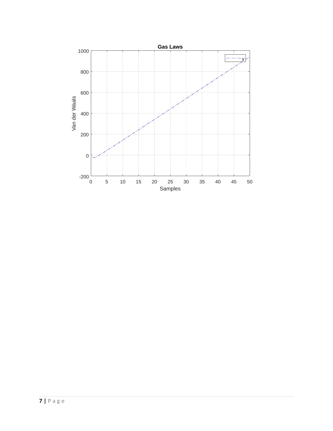
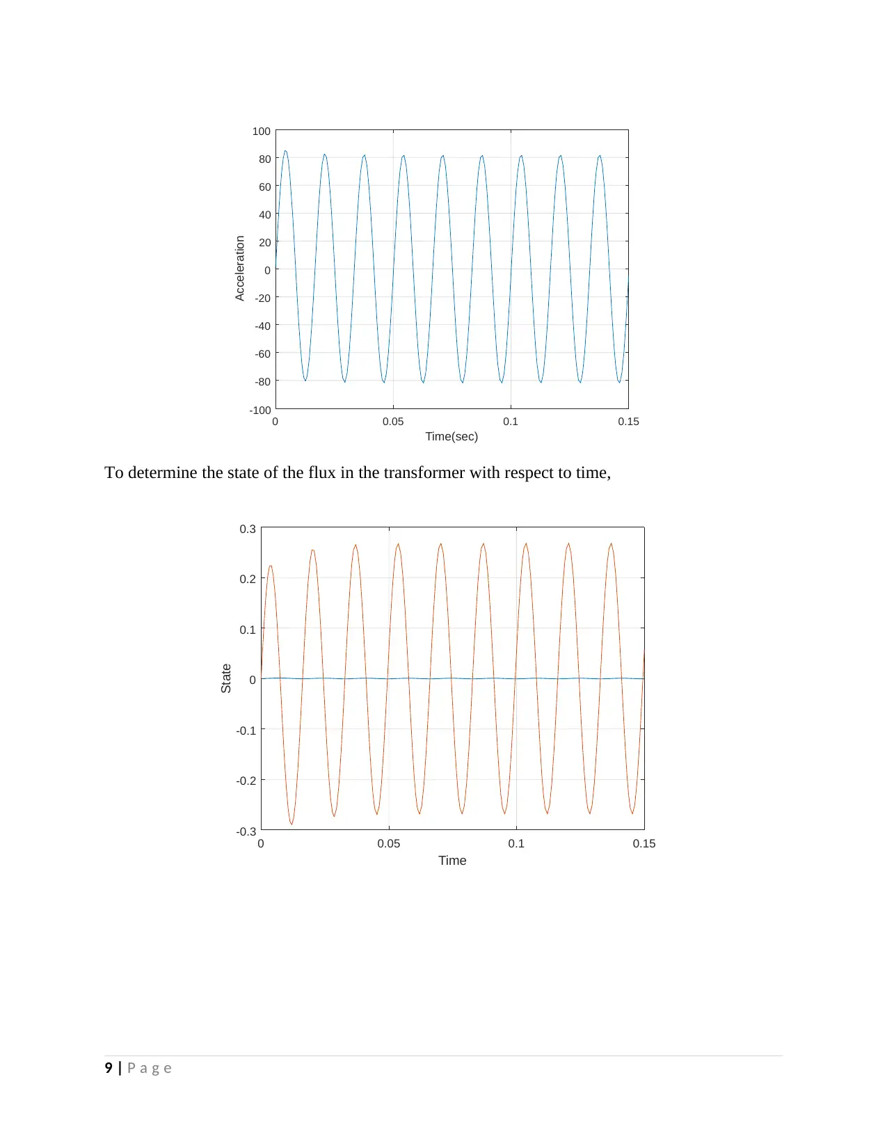
This coursework solution for Numerical Techniques in Engineering (ENGT5140) addresses several key numerical methods. Part A focuses on root-finding using Newton's method, plotting the function, and analyzing convergence. Part B applies Newton's method to a different function, including plotting the function. Question 2 applies Newton's method to the Van der Waals equation to determine molar volumes. Question 12 analyzes the Duffing equation for a transformer's flux, including plotting flux and acceleration versus time. Question 14 implements the shooting method to solve a boundary value problem. The solution includes MATLAB code, plots, and detailed explanations of the methods used.

Institutional affiliation
NUMERICAL TECHNIQUES IN ENGINEERING
ENGT5140
Student ID Number
Student Name
Date of Submission

COURSEWORK QUESTIONS
QUESTION 1
Part A
f ( x )=14 x ex−2−12 ex−2−7 x3 +20 x2 −26 x+12
(i) Plotting the function on the interval [0,3]
Using MATLAB r2018b software, the function is plotted such that,
x=0:0.001:3;
fx=(14*exp(x-2))-(12*exp(x-2))-7*x.^3+20*x.^2-26*x+12;
fx1=diff(fx);
plot(x,fx,'r-.','LineWidth',1.2)
grid on
xlabel('x')
ylabel('f(x)')
0 0.5 1 1.5 2 2.5 3
x
-70
-60
-50
-40
-30
-20
-10
0
10
20
f(x)
(ii) Finding the roots using newton’s method
Using the Newton Raphson Method to find root, the following algorithm is
implemented,
1 | P a g e

% Question 1: Part A:2
fc=@(x) ((14*exp(x-2))-(12*exp(x-2))-7*x.^3+20*x.^2-26*x+12);
xb = fzero(fc,15)
init=20;
tol=1e-2;
maxiter=1e4;
%[root, error_estimate]=newton('fx','fx1',200,tol,maxiter)
function [ x, ex ] = newton( f, df, x0, tol, nmax )
if nargin == 3
tol = 1e-4;
nmax = 1e1;
elseif nargin == 4
nmax = 1e1;
elseif nargin ~= 5
error('newton: invalid input parameters');
end
f = inline(f); %#ok<*DINLN>
df = inline(df);
x(1) = x0 - (f(x0)/df(x0));
ex(1) = abs(x(1)-x0);
k = 2;
while (ex(k-1) >= tol) && (k <= nmax)
x(k) = x(k-1) - (f(x(k-1))/df(x(k-1)));
ex(k) = abs(x(k)-x(k-1));
k = k+1;
end
end
(iii) Finding which roots converge linearly and which ones converge quadratically,
The roots converged linearly as there was a constant value for the roots. There
were however no quadratic roots, as the function is a first order polynomial.
Part B
f ( x )= 3
√1− 3
4 x
(i) Finding the roots of f(x)
%Question 1: Part B
fb=(1-3./(4*x)).^(1/3);
y=abs(fb);
figure(2)
plot(x,y)
2 | P a g e

xlabel('x')
ylabel('f(x)')
grid on
0 0.5 1 1.5 2 2.5 3
x
0
1
2
3
4
5
6
7
8
9
10
f(x)
(ii) Applying the newton’s method on the plot
function [ x, ex ] = newton( f, df, x0, tol, nmax )
if nargin == 3
tol = 1e-4;
nmax = 1e1;
elseif nargin == 4
nmax = 1e1;
elseif nargin ~= 5
error('newton: invalid input parameters');
end
f = inline(f); %#ok<*DINLN>
df = inline(df);
x(1) = x0 - (f(x0)/df(x0));
ex(1) = abs(x(1)-x0);
k = 2;
while (ex(k-1) >= tol) && (k <= nmax)
x(k) = x(k-1) - (f(x(k-1))/df(x(k-1)));
ex(k) = abs(x(k)-x(k-1));
k = k+1;
end
end
3 | P a g e

QUESTION 2
Newton’s method in an application problem for the ideal gas law,
PV =nRT
Using the Van der Waal’s equations,
( P+ n2 a
V 2 ) ( V −nb ) =nRT
The molar volumes for the gases is given as,
v=V
n = RT
p
Temperature, K Pressure, atm Molar Volume,
L/mol
300 1 24.6162
10 2.1416
100 0.2462
500 1 41.0270
10 4.0127
100 0.4103
700 1 57.4378
10 5.7438
100 0.5744
Using the Van Der Waals equation, it is solved as,
( P+ n2 a
V 2 ) ( V −nb ) =nRT
To solve it as,
( P+ a
V 2 ) ( V −nb ) =nRT
To find the zeros or the roots of the function,
4 | P a g e

f ( V )=
(P+ a
V 2 ) ( V −nb )−RT
Using the numerical method to solve for the non-linear equation in the form of f (x)=0
f ' ( V )=P+ a
V 2 − 2 a
V 3 ( V −b )
The Newton-Raphson method approximates a solution to f ( x)=0
f '
( xi )= f ( xi ) −f ( xi+1 )
xi −xi +1
f '
( xi )= f ( xi ) −0
xi−xi +1
→ xi +1=xi− f ( xi )
f '
( xi )
The iterative formula computes the values of the roots up to the approximation to zero for the
function. Implementing the equation on MATLAB,
% v - molar volumes vector
% fg - value of functions at v
R=0.0820578; %molar gas constant
a=1.36; %L^2 atm/mole^2
b=0.003183; %L/mole
P=15; %pressure (atm)
T=320; %one mole of oxygen
v=linspace(0,50);
y=myVanderWaals(v,R,a,b,P,T);
figure(1)
plot(v,y,'r-.')
grid on
v0=ginput(1);
xlabel('Samples')
ylabel('Van der Waals')
title('Gas Laws')
legend('y')
5 | P a g e

0 5 10 15 20 25 30 35 40 45 50
Samples
-100
0
100
200
300
400
500
600
700
800
Van der Waals
Gas Laws
y
Part 2
For the Benzene vapor,
% For Benzene vapor
R=0.0820578; %molar gas constant
a=18.0; %L^2 atm/mole^2
b=0.1154; %L/mole
P=20; %pressure (atm)
T=700; %one mole of oxygen
v=linspace(0,50);
y=myVanderWaals(v,R,a,b,P,T);
figure(1)
plot(v,y,'b-.')
grid on
v0=ginput(1);
xlabel('Samples')
ylabel('Van der Waals')
title('Gas Laws')
legend('y')
6 | P a g e

0 5 10 15 20 25 30 35 40 45 50
Samples
-200
0
200
400
600
800
1000
Van der Waals
Gas Laws
y
7 | P a g e

QUESTION 12
The Duffing equation for the flux in a transformer. The nonlinear differential equation is,
d2 φ
d t2 +ω0
2 φ+b φ3= ω
N E cos ωt φ ( 0 ) =φ' ( 0 )=0
Making a plot of φ versust
clear
tspan = [0 0.15];
c = 83;
val_b = 0.14;
omega = 120*pi;
E=165;
N=600;
A=omega*E/N;
ode_fun = @(t,u,c,val_b,A,omega)[u(2);-u(1)-c*u(2)-
val_b*u(1).^3+A*cos(omega*t)];
[t,u] = ode15s(@(t,u)ode_fun(t,u,c,val_b,A,omega),tspan,[0 0]);
figure(1);
plot(t,u);
xlabel('Time');
ylabel('State');
grid on
acc = -u(:,1)-c*u(:,2)-val_b*u(:,1).^3+A*sin(omega*t);
figure(2);
plot(t,acc);
xlabel('Time(sec)');
ylabel('Acceleration');
grid on
8 | P a g e

0 0.05 0.1 0.15
Time(sec)
-100
-80
-60
-40
-20
0
20
40
60
80
100
Acceleration
To determine the state of the flux in the transformer with respect to time,
0 0.05 0.1 0.15
Time
-0.3
-0.2
-0.1
0
0.1
0.2
0.3
State
9 | P a g e

QUESTION 14
Shooting method to the boundary value problem,
y1
' = 4− y2
t3
y2
' =−e y1
y1 (1 )=0 y2 ( 2 ) =0 , 1≤ t ≤ 2
The shooting method converts the boundary value problem to initial value problem. The
technique performs a trial and error approach to solve the initial value problem. The trial
integrations which are found to satisfy the boundary conditions form part of the endpoints that
are launched [1]-[2]. There is a discrepancy from the desired boundary condition where there are
endpoints that adjust the starting conditions so that the boundary conditions for the different
endpoints are satisfied.
Fk ( V ) =B2 k ( x2 , y ( x2 ) ) k =1,2 , … ,n2
10 | P a g e

The shooting method seeks to determine the roots of F with respect to the independent
variable, V. in the case scenario, to find the roots of Y with reference to t. using the Newton-
Raphson to determine the roots,
0 ≈ Fi ( V +δV ) =Fi ( V ) +∑
l =1
n2
∂ Fi
∂ V l
δ V l+ O ( δ V 2 )
∂ Fi
∂V l
≈ Fi ( V 1 , … , V l+ ∆ V l , … )−Fi ( V 1 , … , V l , … )
∆ V l
% applying the shooting method
[y1, y2]=shooting_method(fun,0.001,1e-5,1,2,[0 0],'fd')
function result_out=fce(y1,y2)
result_out(1)=(4-(y2))/(t^3);
result_out(2)=-exp(y1);
end
The system implements the 4th order Runge Kutta method alongside the shooting method
algorithm to determine the output.
REFERENCES
[1]. H.G. Bock, K.J. Plitt, A Multiple Shooting Algorithm for Direct Solution of Optimal
Control Problems, 1983.
[2]. C. Kirches, H.G. Bock, J.P. Schloder, S. Sager, Complementary condensing for the direct
multiple shooting method, in: Modeling, Simulation and Optimization of Complex
Processes, Springer, 2012, pp. 195–206.
11 | P a g e