ENGT5140 Numerical Techniques in Engineering Solved Assignment

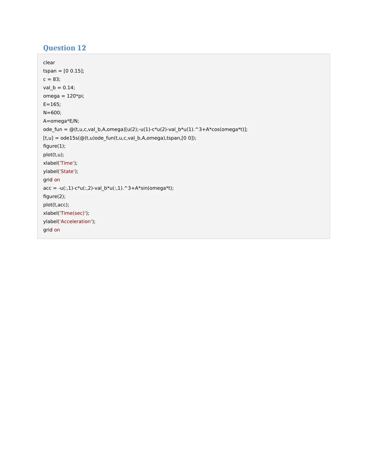
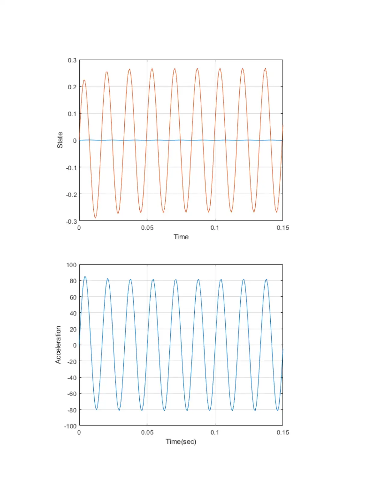
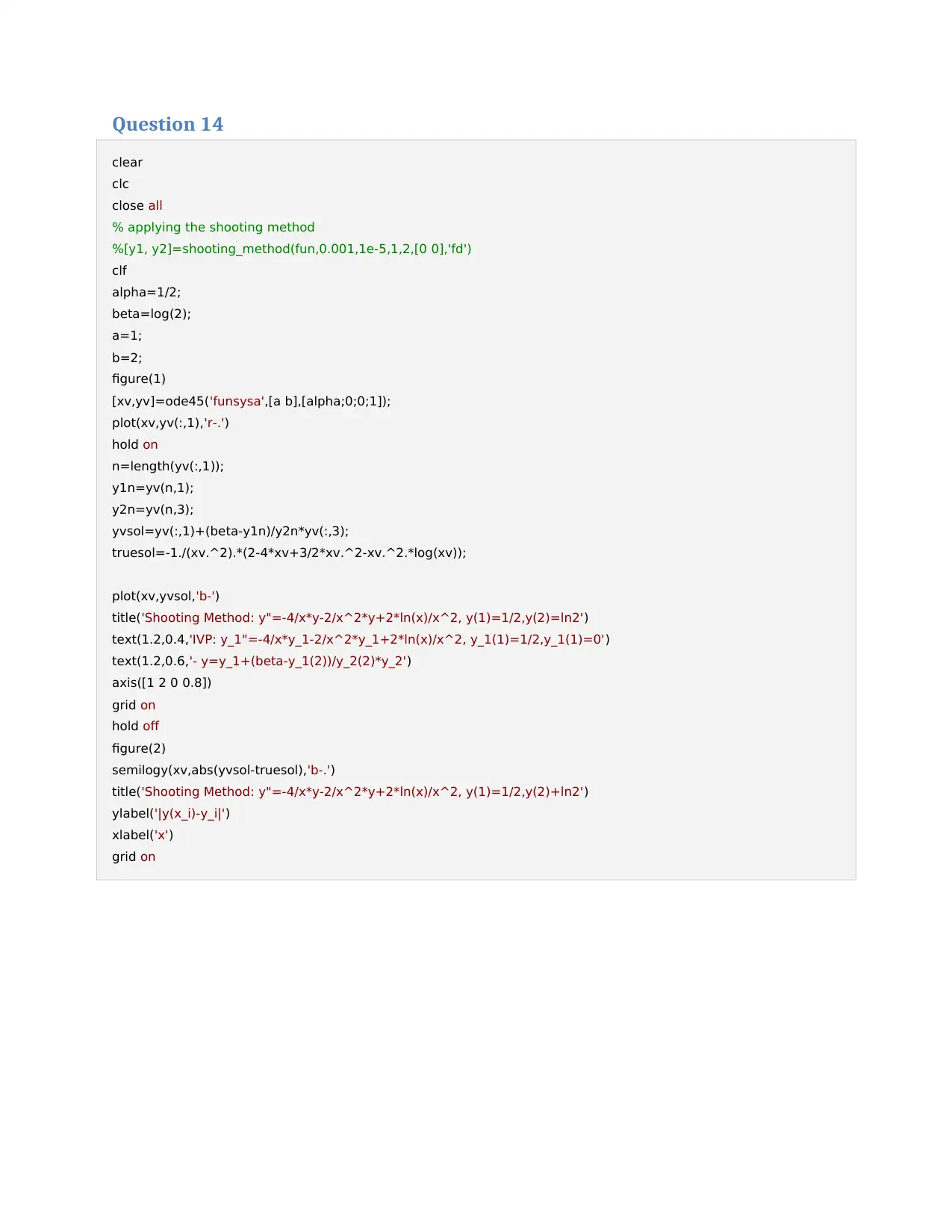
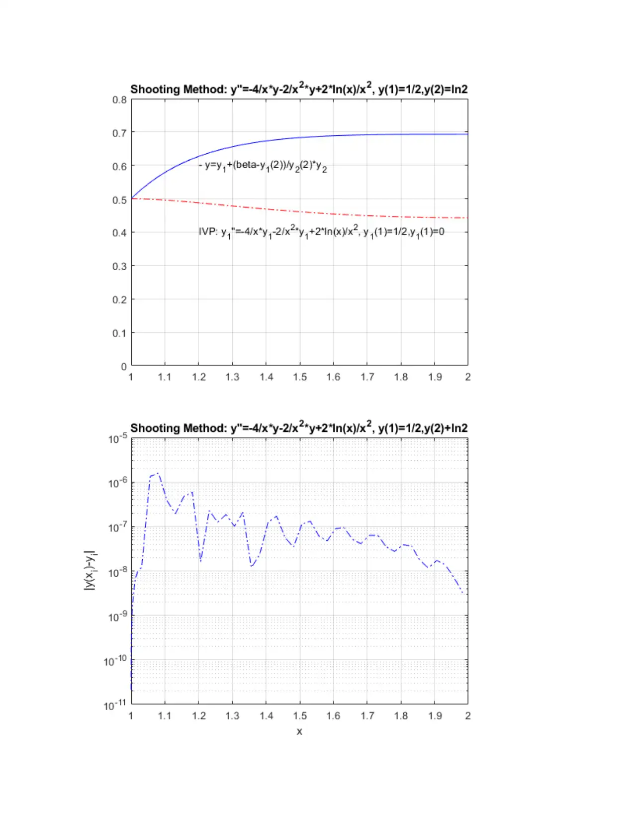
This document presents a solution to a coursework assignment on Numerical Techniques in Engineering (ENGT5140). It includes solutions to four questions involving numerical methods implemented in MATLAB. Question 1 focuses on finding roots of equations using functions like 'fzero' and plotting functions. Question 2 explores Van der Waals equation for oxygen and benzene vapor, plotting the relationship between molar volume and pressure. Question 12 simulates a dynamic system using the 'ode15s' solver and plots the state and acceleration over time. Finally, Question 14 applies the shooting method to solve a second-order boundary value problem, comparing the numerical solution with the true solution. The assignment includes detailed MATLAB code and graphical representations of the results.

CourseWork Questions............................................................................................................................1
Question 1...............................................................................................................................................1
Question 2...............................................................................................................................................3
Question 12.............................................................................................................................................4
Question 14.............................................................................................................................................6
CourseWork Questions
clear all
close all
clc
Question 1
% Question 1: Part A:1
x=0:0.001:3;
fx=(14*exp(x-2))-(12*exp(x-2))-7*x.^3+20*x.^2-26*x+12;
fx1=diff(fx);
plot(x,fx,'r-.','LineWidth',1.2)
grid on
xlabel('x')
ylabel('f(x)')
% Question 1: Part A:2
fc=@(x) ((14*exp(x-2))-(12*exp(x-2))-7*x.^3+20*x.^2-26*x+12);
xb = fzero(fc,15)
init=20;
tol=1e-2;
maxiter=1e4;
%[root, error_estimate]=newton('fx','fx1',200,tol,maxiter)
%Question 1: Part B
fb=(1-3./(4*x)).^(1/3);
y=abs(fb);
figure(2)
plot(x,y)
xlabel('x')
ylabel('f(x)')
grid on
y1=@(x) (1-3/(4*x))^(1/3);
%xc = fzero(y1,15)

xb =
9.8090

Question 2
clear
close all
% v - molar volumes vector
% fg - value of functions at v
%For oxygen
R=0.0820578; %molar gas constant
a=1.36; %L^2 atm/mole^2
b=0.003183; %L/mole
P=15; %pressure (atm)
T=320; %one mole of oxygen
v=linspace(0,50);
y=myVanderWaals(v,R,a,b,P,T);
figure(1)
plot(v,y,'r-.')
grid on
xlabel('Samples')
ylabel('Van der Waals')
title('Gas Laws')

legend('y')
clear
% For Benzene vapor
R=0.0820578; %molar gas constant
a=18.0; %L^2 atm/mole^2
b=0.1154; %L/mole
P=20; %pressure (atm)
T=700; %one mole of oxygen
v=linspace(0,50);
y=myVanderWaals(v,R,a,b,P,T);
figure(1)
plot(v,y,'b-.')
grid on
% v0=ginput(1);
xlabel('Samples')
ylabel('Van der Waals')
title('Gas Laws')
legend('y')

Question 12
clear
tspan = [0 0.15];
c = 83;
val_b = 0.14;
omega = 120*pi;
E=165;
N=600;
A=omega*E/N;
ode_fun = @(t,u,c,val_b,A,omega)[u(2);-u(1)-c*u(2)-val_b*u(1).^3+A*cos(omega*t)];
[t,u] = ode15s(@(t,u)ode_fun(t,u,c,val_b,A,omega),tspan,[0 0]);
figure(1);
plot(t,u);
xlabel('Time');
ylabel('State');
grid on
acc = -u(:,1)-c*u(:,2)-val_b*u(:,1).^3+A*sin(omega*t);
figure(2);
plot(t,acc);
xlabel('Time(sec)');
ylabel('Acceleration');
grid on

Question 14
clear
clc
close all
% applying the shooting method
%[y1, y2]=shooting_method(fun,0.001,1e-5,1,2,[0 0],'fd')
clf
alpha=1/2;
beta=log(2);
a=1;
b=2;
figure(1)
[xv,yv]=ode45('funsysa',[a b],[alpha;0;0;1]);
plot(xv,yv(:,1),'r-.')
hold on
n=length(yv(:,1));
y1n=yv(n,1);
y2n=yv(n,3);
yvsol=yv(:,1)+(beta-y1n)/y2n*yv(:,3);
truesol=-1./(xv.^2).*(2-4*xv+3/2*xv.^2-xv.^2.*log(xv));
plot(xv,yvsol,'b-')
title('Shooting Method: y"=-4/x*y-2/x^2*y+2*ln(x)/x^2, y(1)=1/2,y(2)=ln2')
text(1.2,0.4,'IVP: y_1"=-4/x*y_1-2/x^2*y_1+2*ln(x)/x^2, y_1(1)=1/2,y_1(1)=0')
text(1.2,0.6,'- y=y_1+(beta-y_1(2))/y_2(2)*y_2')
axis([1 2 0 0.8])
grid on
hold off
figure(2)
semilogy(xv,abs(yvsol-truesol),'b-.')
title('Shooting Method: y"=-4/x*y-2/x^2*y+2*ln(x)/x^2, y(1)=1/2,y(2)+ln2')
ylabel('|y(x_i)-y_i|')
xlabel('x')
grid on