Operating System Assignment - Memory Management and Process Scheduling

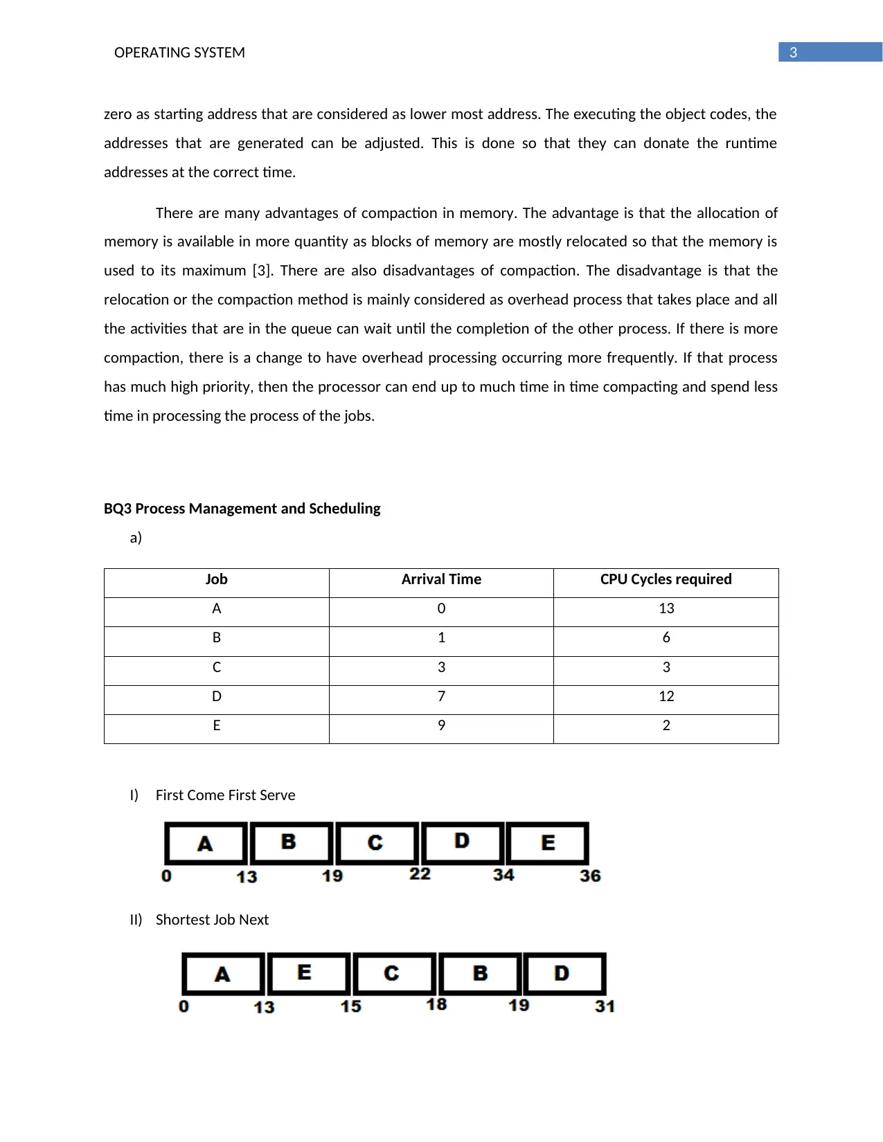
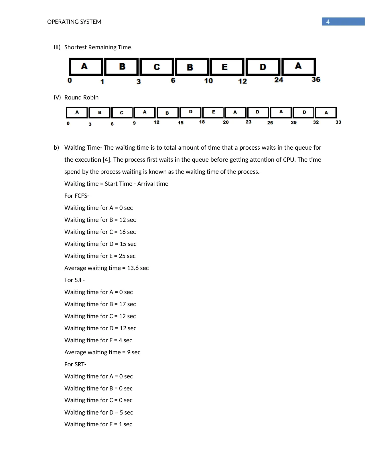
This assignment solution delves into core concepts of operating systems, specifically focusing on memory management and process scheduling. The memory management section explores paging, calculating physical addresses based on logical addresses and frame mappings, and discusses the implications of page availability. It also touches upon the effects of memory compaction on system performance and the trade-offs between fragmentation and relocation. Furthermore, the assignment thoroughly examines process management and scheduling algorithms, including First Come First Serve (FCFS), Shortest Job Next (SJF), Shortest Remaining Time (SRT), and Round Robin. For each algorithm, it calculates waiting time and turnaround time, providing a comparative analysis of their performance metrics. The solution references relevant academic sources to support the analysis and findings.

Running head: OPERATING SYSTEM
Operating System
Name of Student-
Name of University-
Author’s Note-

1OPERATING SYSTEM
BQ1 Memory Management Paging
a. The address at the starting of frame 1 is 1025 and the address at the end of frame 1 is 2048.
b.
1. Yes, page 2 is mapped to frame 2
2. No, page 3 is nor mapped to frame 3. Frame 3 is kept free.
c. Page 3, 6, and 7 are not yet loaded in the memory.
d. When Process A needs and address in page 3, then the paging technique finds the mapping of
page 3 in the frame table. Until the paging process does not respond, the process A has to wait
in the waiting queue for its execution [1]. When the frame is found that is mapped to the page,
then the data is bought to the CPU for its execution. The CPU generates logical address to search
a particular data. In this example, page 3 is not mapped in the frame table. So, the CPU will not
get any data in the main memory.
e.
1. Logical Address- 1023
Memory Size of page and frame table- 1024 bytes
1024 bytes of logical address with 8 pages. Then, each page is of size 1024/8 = 128 bytes
Offset of logical address 1023 % 1024 = 1023
1023/1024 = 0
So, it can be assumed that 1023 is in page 0
Page 0 is mapped to frame number 6
So, the physical address is calculated as
Frame number x Page size + offset
6 * 1024 + 1023 = 7167
So, the physical address is 0001101111111111
2. Logical Address = 3000
Memory Size of page and frame table= 1024 bytes
1024 bytes of logical address with 8 pages. Then, each page is of size 1024/8 = 128 bytes
Offset = 3000 % 1024 = 952
3000/1024 = 2.929
So, it can be assumed that 1023 is in page 2

2OPERATING SYSTEM
Page 2 is mapped to frame number 2
So, the physical address is calculated as
Frame number x Page size + offset
2 * 1024 + 952 = 3000
So, the physical address is 0000101110111000
3. Logical Address- 4120
Memory Size of page and frame table- 1024 bytes
1024 bytes of logical address with 8 pages. Then, each page is of size 1024/8 = 128 bytes
Offset of logical address 4120 % 1024 = 24
1023/1024 = 4.023
So, it can be assumed that 1023 is in page 4
Page 4 is mapped to frame number 1
So, the physical address is calculated as
Frame number x Page size + offset
1 * 1024 + 24 = 1048
So, the physical address is 0000010000011000
4. Logical Address- 5000
Memory Size of page and frame table- 1024 bytes
1024 bytes of logical address with 8 pages. Then, each page is of size 1024/8 = 128 bytes
Offset of logical address = 5000 % 1024 = 904
5000/1024 = 4.882
So, it can be assumed that 1023 is in page 4
Page 4 is mapped to frame number 1
So, the physical address is calculated as
Frame number x Page size + offset
1 * 1024 + 904 = 1028
So, the physical address is 0000011110001000
BQ2 Fragmentation and Memory Mapping
Relocation or compaction of memory can be performed before running of any of the programs
in the system [2]. The assemblers and the compilers are generated typically which are executed with

3OPERATING SYSTEM
zero as starting address that are considered as lower most address. The executing the object codes, the
addresses that are generated can be adjusted. This is done so that they can donate the runtime
addresses at the correct time.
There are many advantages of compaction in memory. The advantage is that the allocation of
memory is available in more quantity as blocks of memory are mostly relocated so that the memory is
used to its maximum [3]. There are also disadvantages of compaction. The disadvantage is that the
relocation or the compaction method is mainly considered as overhead process that takes place and all
the activities that are in the queue can wait until the completion of the other process. If there is more
compaction, there is a change to have overhead processing occurring more frequently. If that process
has much high priority, then the processor can end up to much time in time compacting and spend less
time in processing the process of the jobs.
BQ3 Process Management and Scheduling
a)
Job Arrival Time CPU Cycles required
A 0 13
B 1 6
C 3 3
D 7 12
E 9 2
I) First Come First Serve
II) Shortest Job Next

4OPERATING SYSTEM
III) Shortest Remaining Time
IV) Round Robin
b) Waiting Time- The waiting time is to total amount of time that a process waits in the queue for
the execution [4]. The process first waits in the queue before getting attention of CPU. The time
spend by the process waiting is known as the waiting time of the process.
Waiting time = Start Time - Arrival time
For FCFS-
Waiting time for A = 0 sec
Waiting time for B = 12 sec
Waiting time for C = 16 sec
Waiting time for D = 15 sec
Waiting time for E = 25 sec
Average waiting time = 13.6 sec
For SJF-
Waiting time for A = 0 sec
Waiting time for B = 17 sec
Waiting time for C = 12 sec
Waiting time for D = 12 sec
Waiting time for E = 4 sec
Average waiting time = 9 sec
For SRT-
Waiting time for A = 0 sec
Waiting time for B = 0 sec
Waiting time for C = 0 sec
Waiting time for D = 5 sec
Waiting time for E = 1 sec

5OPERATING SYSTEM
Average waiting time = 1.2 sec
For Round Robin
Waiting time for A = 0 sec
Waiting time for B = 2 sec
Waiting time for C = 3 sec
Waiting time for D = 8 sec
Waiting time for E = 9 sec
Average waiting time = 4.4 sec
Turn Around Time- The total Turn Around Time for a process if the time a process takes from the
submission of the process to its complete execution [5].
Turn Around Time = Burst Time + Waiting Time
For FCFS-
Turn Around Time for A = 13 sec
Turn Around Time for B = 18 sec
Turn Around Time for C = 19 sec
Turn Around Time for D = 27 sec
Turn Around Time for E = 27 sec
Average Turn Around Time = 20.8 sec
For SJF-
Turn Around Time for A = 13 sec
Turn Around Time for B = 23 sec
Turn Around Time for C = 15 sec
Turn Around Time for D = 24 sec
Turn Around Time for E = 6 sec
Average Turn Around Time = 16.2 sec
For SRT-
Turn Around Time for A = 13 sec
Turn Around Time for B = 6 sec
Turn Around Time for C = 3 sec
Turn Around Time for D = 17 sec
Turn Around Time for E = 3 sec
Average Turn Around Time = 7.8 sec

6OPERATING SYSTEM
For Round Robin
Turn Around Time for A = 13 sec
Turn Around Time for B = 8 sec
Turn Around Time for C = 6 sec
Turn Around Time for D = 20 sec
Turn Around Time for E = 11 sec
Average Turn Around Time = 11.6 sec
References
[1] Oren, Gal, Leonid Barenboim, and Lior Amar. "Memory-Aware Management for Heterogeneous
Main Memory Using an Optimization of the Aging Paging Algorithm." In Parallel Processing
Workshops (ICPPW), 2016 45th International Conference on, pp. 98-105. IEEE, 2016.
[2] Boyar, Joan, Sushmita Gupta, and Kim S. Larsen. "Relative interval analysis of paging algorithms
on access graphs." Theoretical Computer Science 568 (2015): 28-48.
[3] Wang, K. C. "Memory Management." In Design and Implementation of the MTX Operating
System, pp. 215-234. Springer International Publishing, 2015.
[4] Arabnejad, Hamid, and Jorge G. Barbosa. "List scheduling algorithm for heterogeneous systems
by an optimistic cost table." IEEE Transactions on Parallel and Distributed Systems25, no. 3
(2014): 682-694.
[5] Kumari, Rajani, Vivek Kumar Sharma, and Sandeep Kumar. "Design and Implementation of
Modified Fuzzy based CPU Scheduling Algorithm." arXiv preprint arXiv:1706.02621(2017).