Operations Management: Inventory, Forecasting, and Production Plan

This report provides an analysis of operations management principles, focusing on inventory management, demand forecasting, and production planning. It begins with a discussion of purchasing and shortage costs associated with inventory, including purchase cost and opportunity cost. The report then calculates and compares the total costs of different inventory plans (Plan A, B, C, D) and determines the Economic Order Quantity (EOQ) in Plan E. Furthermore, it forecasts quarterly sales using seasonal indices and discusses qualitative and quantitative forecasting methods. Finally, the report completes level and chase production plans for a six-month period, recommending the chase production plan for better alignment with market demand. The analysis aims to optimize inventory levels, improve forecasting accuracy, and enhance production efficiency.

OPERATIONS
MANAGEMENT

Table of Contents
INTRODUCTION...........................................................................................................................3
REFERENCES................................................................................................................................1

Question 1
(a) Discussion of purchasing and shortage cost associated with inventory management
Aside of ordering and holding cost, the two cost which is need to be address by the
company for the management of the inventory includes purchase cost and opportunity cost.
 Purchase cost: The purchase cost is the cost which company will incur while ordering
and purchasing the annual requirement of raw material. The purchase price plays
important role in this because the purchase price of the raw material change and also
affects the holding cost of the inventory. The purchase cost also involves the purchase
price of the raw material, the production cost if such material is produced within the
organisation. The price may remain constant and also vary depends upon the number of
quantity of raw material.
 Opportunity cost: This is another cost which is important and associated with the
company inventory management. This cost involves the other cost which the company
will lose in term to keep this plan in active. The opportunity cost involves the range of
investment alternatives, lack of capital availability that they need to invest in alternatives
and related cost to the overall role of inventory within the logistic system. This cost play
important role in deciding the optimal quantity that company need to order at a particular
point of time.
(b) Calculation of total cost of Plan A and Plan B
Particulars Plan A Plan B
Order Quantities 200 Units 50 Units
Annual Demand 350 Units 350 Units
Holding cost per unit £0.8 £0.8
Ordering cost per order £12.5 £12.5
No of order placed in a
year
350 / 200 = 1.75 orders 350 / 50 = 7 orders
Average Inventory 200 / 2 = 100 units 50 / 2 = 25 units
Calculation of Total cost of Plan A and Plan B

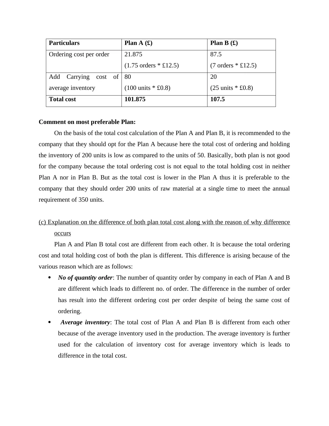
Particulars Plan A (£) Plan B (£)
Ordering cost per order 21.875
(1.75 orders * £12.5)
87.5
(7 orders * £12.5)
Add Carrying cost of
average inventory
80
(100 units * £0.8)
20
(25 units * £0.8)
Total cost 101.875 107.5
Comment on most preferable Plan:
On the basis of the total cost calculation of the Plan A and Plan B, it is recommended to the
company that they should opt for the Plan A because here the total cost of ordering and holding
the inventory of 200 units is low as compared to the units of 50. Basically, both plan is not good
for the company because the total ordering cost is not equal to the total holding cost in neither
Plan A nor in Plan B. But as the total cost is lower in the Plan A thus it is preferable to the
company that they should order 200 units of raw material at a single time to meet the annual
requirement of 350 units.
(c) Explanation on the difference of both plan total cost along with the reason of why difference
occurs
Plan A and Plan B total cost are different from each other. It is because the total ordering
cost and total holding cost of both the plan is different. This difference is arising because of the
various reason which are as follows:
 No of quantity order: The number of quantity order by company in each of Plan A and B
are different which leads to different no. of order. The difference in the number of order
has result into the different ordering cost per order despite of being the same cost of
ordering.
 Average inventory: The total cost of Plan A and Plan B is different from each other
because of the average inventory used in the production. The average inventory is further
used for the calculation of inventory cost for average inventory which is leads to
difference in the total cost.

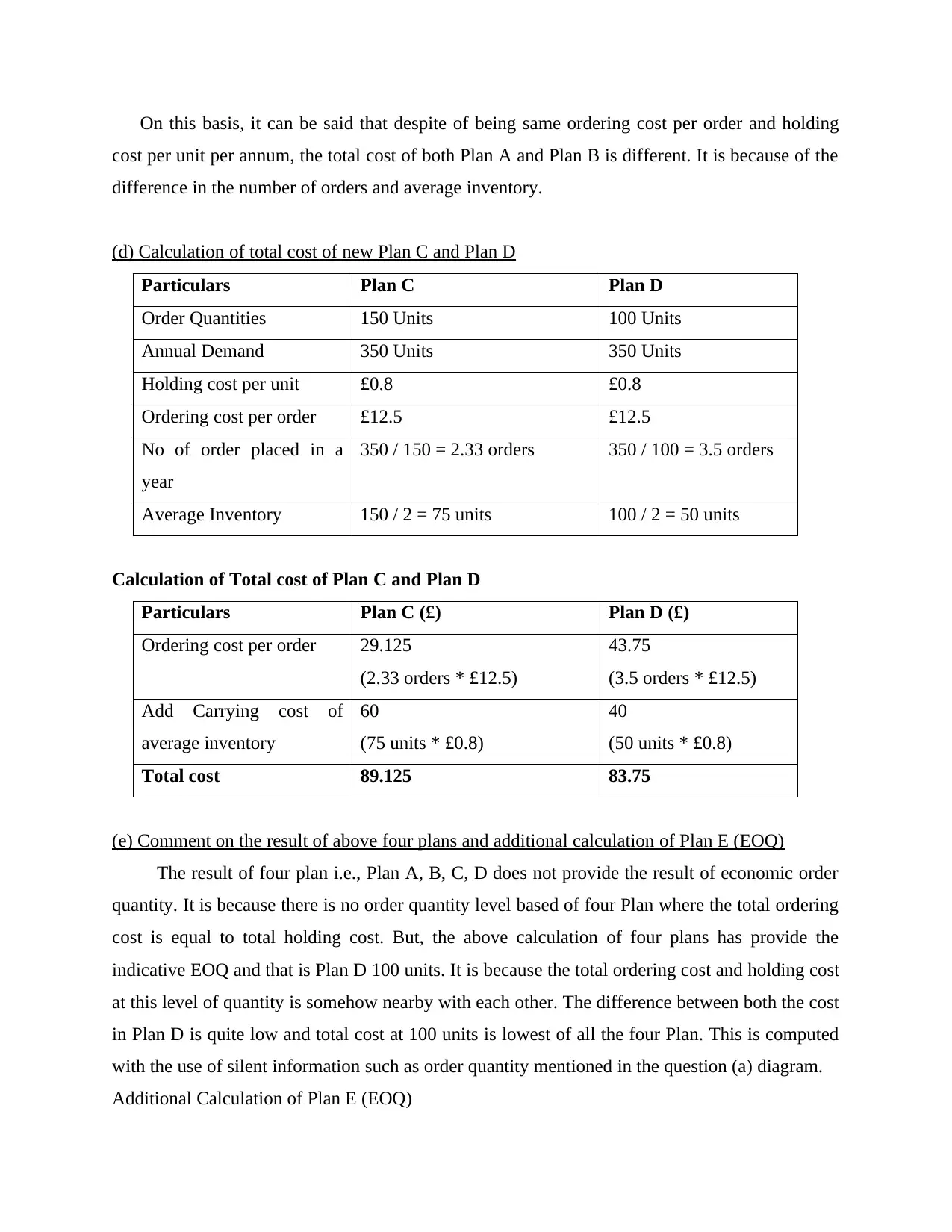
On this basis, it can be said that despite of being same ordering cost per order and holding
cost per unit per annum, the total cost of both Plan A and Plan B is different. It is because of the
difference in the number of orders and average inventory.
(d) Calculation of total cost of new Plan C and Plan D
Particulars Plan C Plan D
Order Quantities 150 Units 100 Units
Annual Demand 350 Units 350 Units
Holding cost per unit £0.8 £0.8
Ordering cost per order £12.5 £12.5
No of order placed in a
year
350 / 150 = 2.33 orders 350 / 100 = 3.5 orders
Average Inventory 150 / 2 = 75 units 100 / 2 = 50 units
Calculation of Total cost of Plan C and Plan D
Particulars Plan C (£) Plan D (£)
Ordering cost per order 29.125
(2.33 orders * £12.5)
43.75
(3.5 orders * £12.5)
Add Carrying cost of
average inventory
60
(75 units * £0.8)
40
(50 units * £0.8)
Total cost 89.125 83.75
(e) Comment on the result of above four plans and additional calculation of Plan E (EOQ)
The result of four plan i.e., Plan A, B, C, D does not provide the result of economic order
quantity. It is because there is no order quantity level based of four Plan where the total ordering
cost is equal to total holding cost. But, the above calculation of four plans has provide the
indicative EOQ and that is Plan D 100 units. It is because the total ordering cost and holding cost
at this level of quantity is somehow nearby with each other. The difference between both the cost
in Plan D is quite low and total cost at 100 units is lowest of all the four Plan. This is computed
with the use of silent information such as order quantity mentioned in the question (a) diagram.
Additional Calculation of Plan E (EOQ)

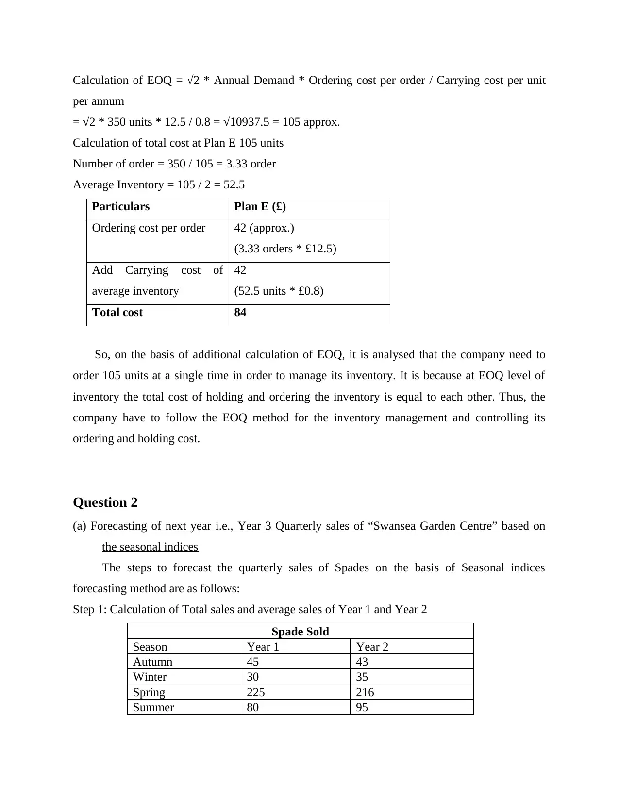
Calculation of EOQ = √2 * Annual Demand * Ordering cost per order / Carrying cost per unit
per annum
= √2 * 350 units * 12.5 / 0.8 = √10937.5 = 105 approx.
Calculation of total cost at Plan E 105 units
Number of order = 350 / 105 = 3.33 order
Average Inventory = 105 / 2 = 52.5
Particulars Plan E (£)
Ordering cost per order 42 (approx.)
(3.33 orders * £12.5)
Add Carrying cost of
average inventory
42
(52.5 units * £0.8)
Total cost 84
So, on the basis of additional calculation of EOQ, it is analysed that the company need to
order 105 units at a single time in order to manage its inventory. It is because at EOQ level of
inventory the total cost of holding and ordering the inventory is equal to each other. Thus, the
company have to follow the EOQ method for the inventory management and controlling its
ordering and holding cost.
Question 2
(a) Forecasting of next year i.e., Year 3 Quarterly sales of “Swansea Garden Centre” based on
the seasonal indices
The steps to forecast the quarterly sales of Spades on the basis of Seasonal indices
forecasting method are as follows:
Step 1: Calculation of Total sales and average sales of Year 1 and Year 2
Spade Sold
Season Year 1 Year 2
Autumn 45 43
Winter 30 35
Spring 225 216
Summer 80 95

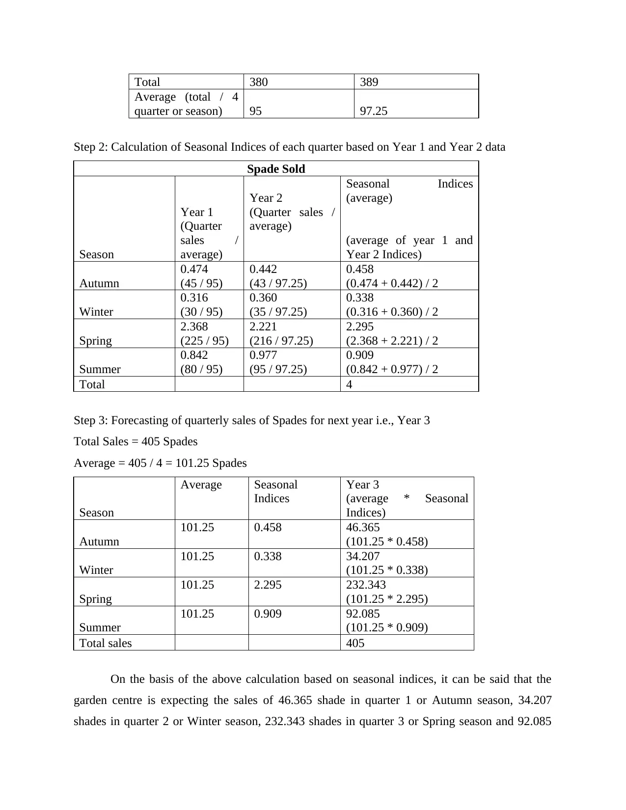
Total 380 389
Average (total / 4
quarter or season) 95 97.25
Step 2: Calculation of Seasonal Indices of each quarter based on Year 1 and Year 2 data
Spade Sold
Season
Year 1
(Quarter
sales /
average)
Year 2
(Quarter sales /
average)
Seasonal Indices
(average)
(average of year 1 and
Year 2 Indices)
Autumn
0.474
(45 / 95)
0.442
(43 / 97.25)
0.458
(0.474 + 0.442) / 2
Winter
0.316
(30 / 95)
0.360
(35 / 97.25)
0.338
(0.316 + 0.360) / 2
Spring
2.368
(225 / 95)
2.221
(216 / 97.25)
2.295
(2.368 + 2.221) / 2
Summer
0.842
(80 / 95)
0.977
(95 / 97.25)
0.909
(0.842 + 0.977) / 2
Total 4
Step 3: Forecasting of quarterly sales of Spades for next year i.e., Year 3
Total Sales = 405 Spades
Average = 405 / 4 = 101.25 Spades
Season
Average Seasonal
Indices
Year 3
(average * Seasonal
Indices)
Autumn
101.25 0.458 46.365
(101.25 * 0.458)
Winter
101.25 0.338 34.207
(101.25 * 0.338)
Spring
101.25 2.295 232.343
(101.25 * 2.295)
Summer
101.25 0.909 92.085
(101.25 * 0.909)
Total sales 405
On the basis of the above calculation based on seasonal indices, it can be said that the
garden centre is expecting the sales of 46.365 shade in quarter 1 or Autumn season, 34.207
shades in quarter 2 or Winter season, 232.343 shades in quarter 3 or Spring season and 92.085

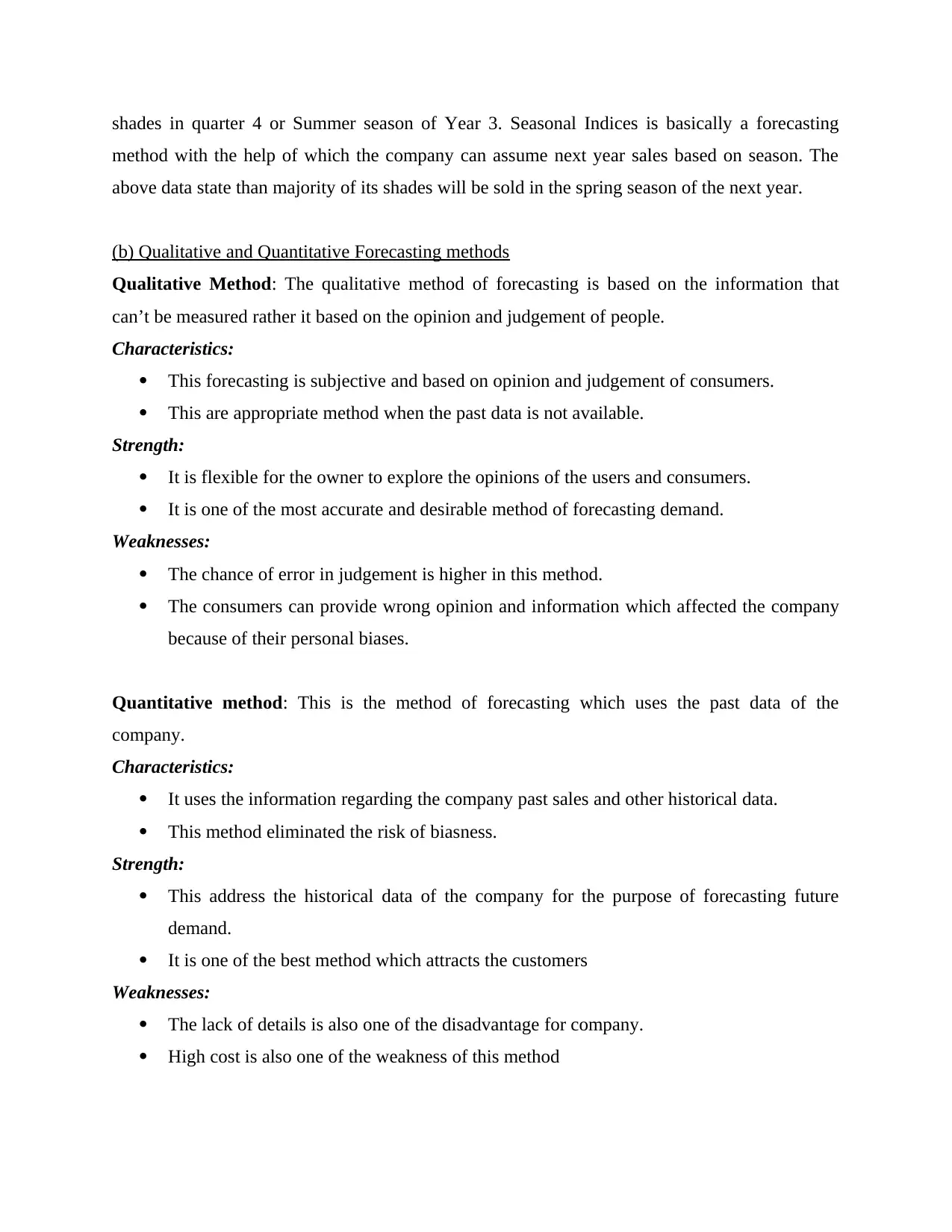
shades in quarter 4 or Summer season of Year 3. Seasonal Indices is basically a forecasting
method with the help of which the company can assume next year sales based on season. The
above data state than majority of its shades will be sold in the spring season of the next year.
(b) Qualitative and Quantitative Forecasting methods
Qualitative Method: The qualitative method of forecasting is based on the information that
can’t be measured rather it based on the opinion and judgement of people.
Characteristics:
 This forecasting is subjective and based on opinion and judgement of consumers.
 This are appropriate method when the past data is not available.
Strength:
 It is flexible for the owner to explore the opinions of the users and consumers.
 It is one of the most accurate and desirable method of forecasting demand.
Weaknesses:
 The chance of error in judgement is higher in this method.
 The consumers can provide wrong opinion and information which affected the company
because of their personal biases.
Quantitative method: This is the method of forecasting which uses the past data of the
company.
Characteristics:
 It uses the information regarding the company past sales and other historical data.
 This method eliminated the risk of biasness.
Strength:
 This address the historical data of the company for the purpose of forecasting future
demand.
 It is one of the best method which attracts the customers
Weaknesses:
 The lack of details is also one of the disadvantage for company.
 High cost is also one of the weakness of this method

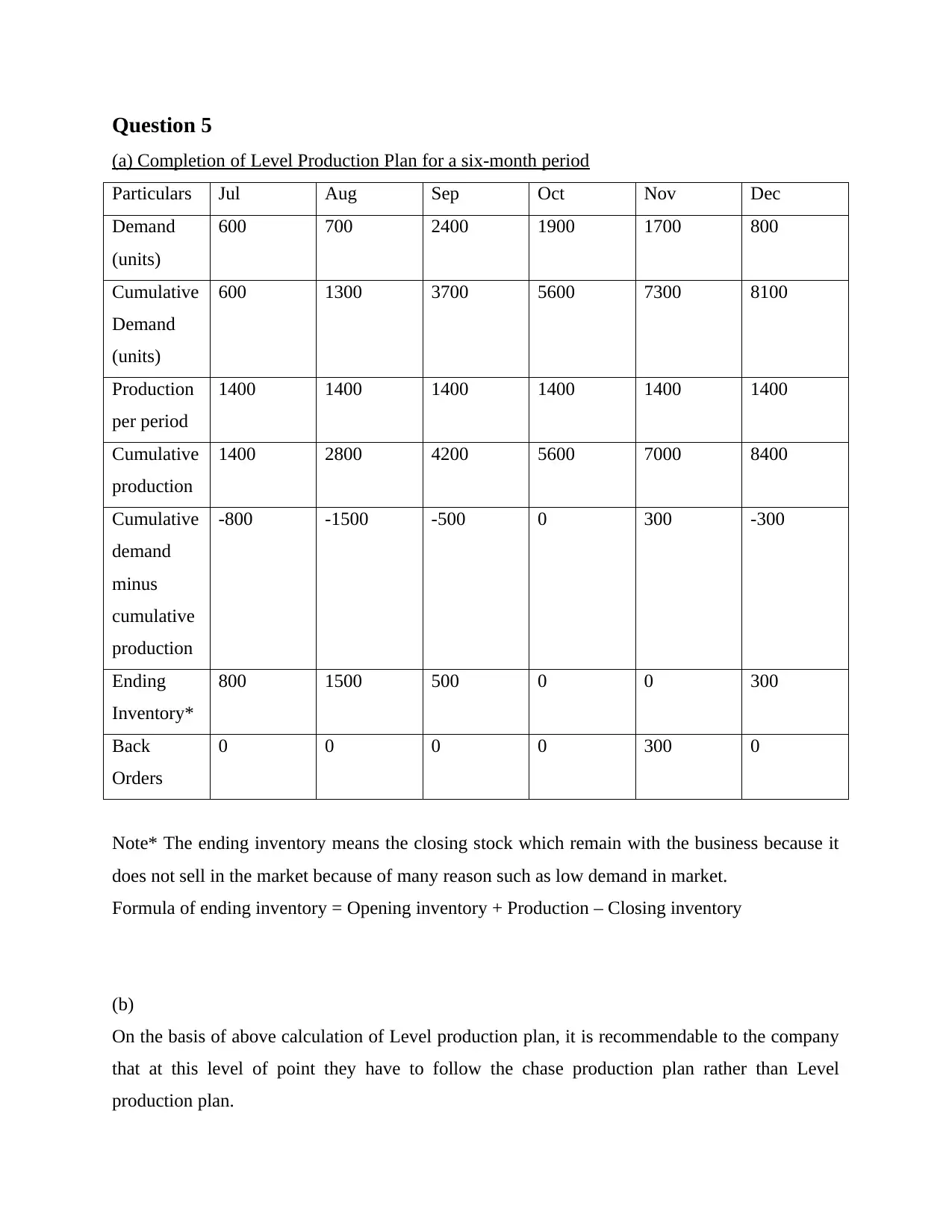
Question 5
(a) Completion of Level Production Plan for a six-month period
Particulars Jul Aug Sep Oct Nov Dec
Demand
(units)
600 700 2400 1900 1700 800
Cumulative
Demand
(units)
600 1300 3700 5600 7300 8100
Production
per period
1400 1400 1400 1400 1400 1400
Cumulative
production
1400 2800 4200 5600 7000 8400
Cumulative
demand
minus
cumulative
production
-800 -1500 -500 0 300 -300
Ending
Inventory*
800 1500 500 0 0 300
Back
Orders
0 0 0 0 300 0
Note* The ending inventory means the closing stock which remain with the business because it
does not sell in the market because of many reason such as low demand in market.
Formula of ending inventory = Opening inventory + Production – Closing inventory
(b)
On the basis of above calculation of Level production plan, it is recommendable to the company
that at this level of point they have to follow the chase production plan rather than Level
production plan.

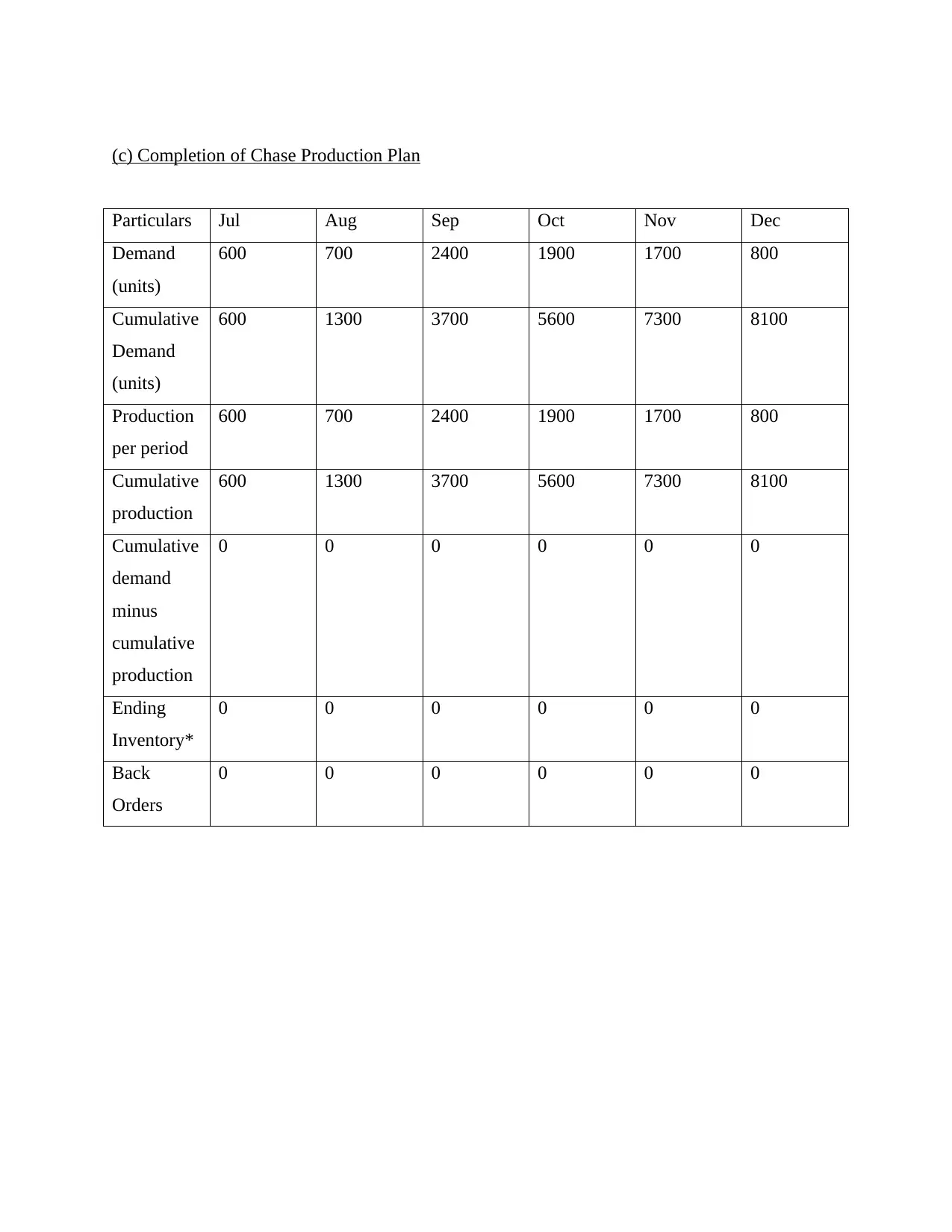
(c) Completion of Chase Production Plan
Particulars Jul Aug Sep Oct Nov Dec
Demand
(units)
600 700 2400 1900 1700 800
Cumulative
Demand
(units)
600 1300 3700 5600 7300 8100
Production
per period
600 700 2400 1900 1700 800
Cumulative
production
600 1300 3700 5600 7300 8100
Cumulative
demand
minus
cumulative
production
0 0 0 0 0 0
Ending
Inventory*
0 0 0 0 0 0
Back
Orders
0 0 0 0 0 0

(d)
The chase plan is more suitable fro the business as this involve the level of expected
demand in market while delivering production practices in business. The total expected demand
in market rise will further influence to the production plan. Management can control the
production on the basis to the expected demand in the market. As the production practice involve
the cost structure swell. If the company produce more than the quantity demanded in market than
this would further include additional cost of worker, hiring cost, inventory cost and such other
cost (Ismailova, 2019). As the quantity produce by per worker is certain and in case of extra
production is practice than the management will be require to appoint one more worker that will
cost 200. Chase plan is more favourable in nature as it allow the organisation to set the quantity
produced and production process on the basis of the total expected demand in the market. The
chase plan will allow the management to implement the production on the basis of the total
estimated quantity demanded in the market. Chase plan is suitable as it allow the organisation to
control the production cycle on the basis to the expected quantity demanded in the market. As
the production will consider different type of cost which involve worker cost, holding cost,
hiring cost and such other.
Question 6
(a)
Operation management is a process of managing the operational requirement of the
business. The role of operation management is to support business house by ensuring all the need
and demand of the company related to its operation management practice,. Over the past century
every operation and functional area of the business could get more professional. Skilled
workforce has been deployed over every single functional activity. In such a time the role of
operation management has also improved (Bazmohammadi and et.al., 2018). The concept of
operation management has recently been advanced in the business environment. The operation
management involve different practices that comprise with the planning; organising, staffing,
leading and controlling the operations perform by the organisation. Every functional and
operational area in the theory is well supported for the management to support the operations of
the business. Over the past century the operation management has developed immensely as a
1

concept. This become more professional and techniques become a part of each stage of the
operation management function in business. The practice of the operation management is well
advanced and developed in the last one century. Many concept have emerged in the entire
century which could bring more proficiencies to the approach of operation management in the
business.
In the current business environment there are plenty of influence factors become a part of
the approach of operation management in business which include political factor, economic,
social, technological, environment and legal factors that are also a part of the approach of
operation management followed by the businesses. Earlier the entire area of operation
management was not advanced. Over the period the transformation took place in the operation
management practice and the businesses practice this entire approach in more efficient manner
(Albert, 2020). The role of the operation management becomes cost in the current time. Various
influencing factors like technology that could completely change to the entire practice of
operation management. The inclusion of technology could make it more advanced and developed
for the business that has further supported to the management to support the overall practice of
operation management in business. Technology has been one of the major influencing factor that
could completely change the entire synergy of operation management practice in business.
Economic factor is another suitable and influencing factor of the current business environment
that could favour the operation management practice in the business. This factor could provide
better environment to the management to allocate suitable resources in order to practice well
advanced and developed practices related to operation management in business.
(b)
Philosophy of lean production with the six central tenets are classify with the use of
certain aspects. Map the value stream is the first and foremost factor or element that support to
the lean production approach. Map the value stream is comprises with the features like
production process, material information and the work flows should be diagrammed to determine
the current state of operations. Flow processing is another aspect and philosophy of the lean
production. Flow processes is about to understand the flow of production and based on that make
a suitable plan to support the best outcome possible. Make what is necessary is another suitable
aspect of the lean production. These consider the fact that the organisation must produce the
product or services that are necessary to develop. This will allow the management to support the
2