Operations Management Systems Pre-Lecture Questions - UniSA Assignment
VerifiedAdded on 2022/11/18
|19
|4994
|233
Homework Assignment
AI Summary
This document presents a comprehensive overview of operations management, addressing key concepts through pre-lecture questions and answers. It explores operations as a transformation process, major decision-making processes, and the competitiveness of business organizations, alongside productivity measurement. The assignment delves into quality control, discussing determinants, costs, and quality-productivity ratios, including the use of control charts. It further covers aggregate planning, strategies, and available-to-promise inventory, extending to material requirement planning (MRP), lean operations, and JIT systems. The content also touches on line balancing, job design, and stopwatch time studies, providing a broad understanding of operational strategies, competitiveness, and productivity within the context of a university assignment.
Pre-lecture Questions
UNIVERSITY OF SOUTH AUSTRALIA
SCHOOL OF ENGINEERING
Operation Management Systems
Student Name:
Student ID Number:
Submission Date:
UNIVERSITY OF SOUTH AUSTRALIA
SCHOOL OF ENGINEERING
Operation Management Systems
Student Name:
Student ID Number:
Submission Date:
Paraphrase This Document
Need a fresh take? Get an instant paraphrase of this document with our AI Paraphraser
Table of Contents
(1) Operations as a transformation process................................................................................4
(2) Major decision-making processes........................................................................................4
(3) Competitiveness of business organisation............................................................................4
(4) Productivity..........................................................................................................................5
(5) Influence of non-economic factors on make-or-buy decisions............................................5
(6) Types of processes................................................................................................................5
(7) Line balancing......................................................................................................................6
(8) Job design and methods analysis..........................................................................................7
(9) Stopwatch time study...........................................................................................................8
(10) Determinants of quality......................................................................................................8
(11) Costs of quality...................................................................................................................9
(12) Quality-productivity ratio...................................................................................................9
(13) Control chart: c-chart..........................................................................................................9
(14) Run chart..........................................................................................................................10
(15) Aggregate planning..........................................................................................................12
(16) Strategies of aggregate planning......................................................................................12
(17) Available-to-promise inventory........................................................................................12
(18) Rough-cut capacity planning............................................................................................13
(19) Material Requirement Planning MRP I............................................................................13
(20) MRP: Outputs...................................................................................................................13
(21) Lot sizing in MRP processing..........................................................................................13
(22) Capacity requirement planning.........................................................................................13
(23) MRP II and ERP...............................................................................................................14
(24) Ultimate goal of lean operation........................................................................................14
(25) Waste in lean systems.......................................................................................................14
(26) Design and operation of lean system................................................................................15
(27) SMED (Single-minute exchange of die) relation with lean operation.............................15
(28) Difference between push systems and pull systems.........................................................15
(29) Kanban Calculation..........................................................................................................16
(30) Significance of Operation Management...........................................................................16
References................................................................................................................................18
List of Tables
Table 1: Measurement of productivity source: Reid, and Sanders (2015)............................5
Table 2: Calculation of positional weights per task (source: PANNEERSELVAM, 2012)....7
Table 3: Assigning the work stations.........................................................................................7
Table 4: Stopwatch time study...................................................................................................8
Table 5: Control chart limits (Source: Madu, 2012)..............................................................10
Table 6: Run chart table (Source: Rumane, 2017)................................................................11
Table 7: Available-to-promise inventory (Source: Wild, 2017)..............................................12
List of Figures
Figure 1: Precedence diagram....................................................................................................6
Figure 2: C-chart diagram........................................................................................................10
⊘ This is a preview!⊘
Do you want full access?
Subscribe today to unlock all pages.
Trusted by 1+ million students worldwide
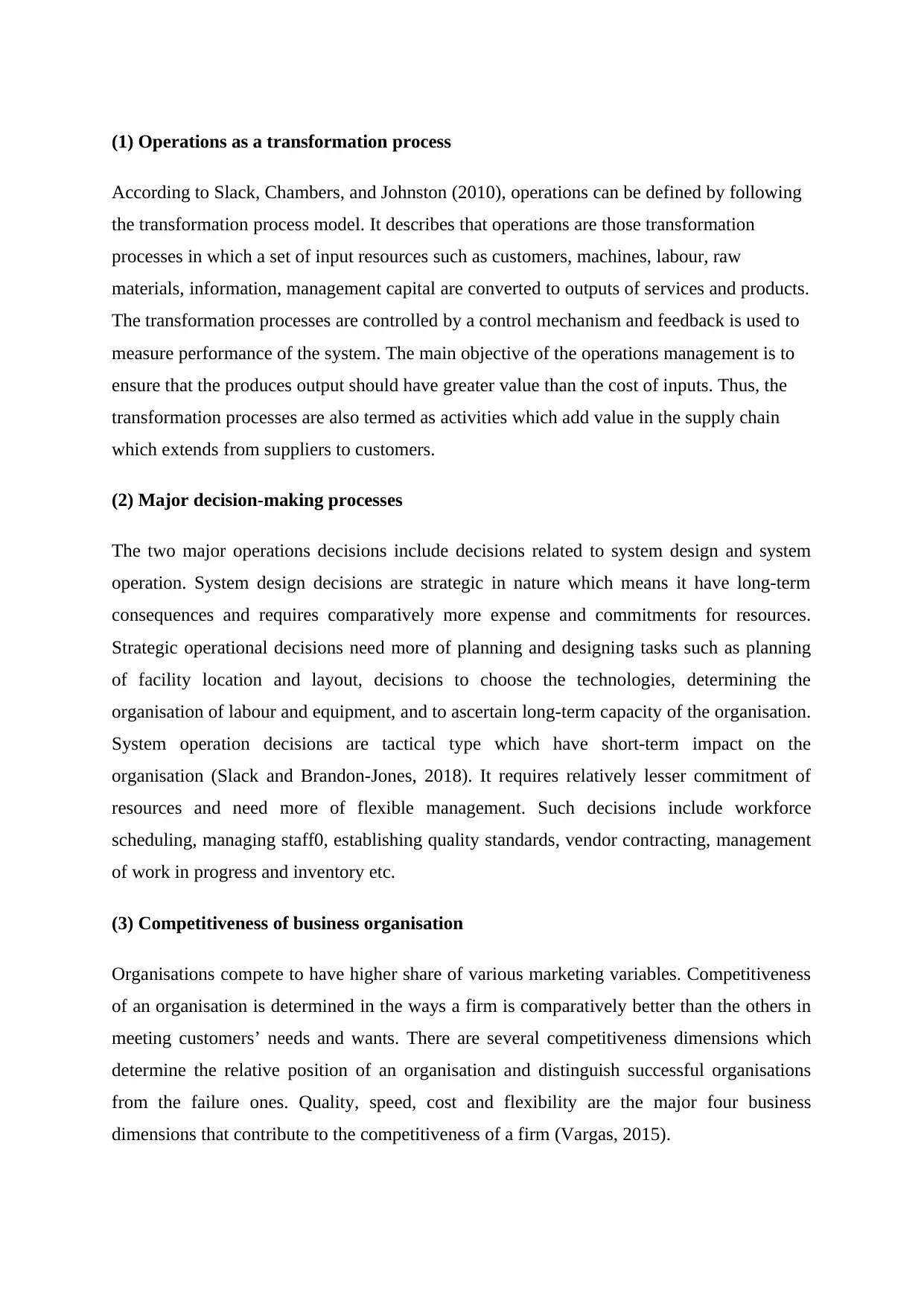
(1) Operations as a transformation process
According to Slack, Chambers, and Johnston (2010), operations can be defined by following
the transformation process model. It describes that operations are those transformation
processes in which a set of input resources such as customers, machines, labour, raw
materials, information, management capital are converted to outputs of services and products.
The transformation processes are controlled by a control mechanism and feedback is used to
measure performance of the system. The main objective of the operations management is to
ensure that the produces output should have greater value than the cost of inputs. Thus, the
transformation processes are also termed as activities which add value in the supply chain
which extends from suppliers to customers.
(2) Major decision-making processes
The two major operations decisions include decisions related to system design and system
operation. System design decisions are strategic in nature which means it have long-term
consequences and requires comparatively more expense and commitments for resources.
Strategic operational decisions need more of planning and designing tasks such as planning
of facility location and layout, decisions to choose the technologies, determining the
organisation of labour and equipment, and to ascertain long-term capacity of the organisation.
System operation decisions are tactical type which have short-term impact on the
organisation (Slack and Brandon-Jones, 2018). It requires relatively lesser commitment of
resources and need more of flexible management. Such decisions include workforce
scheduling, managing staff0, establishing quality standards, vendor contracting, management
of work in progress and inventory etc.
(3) Competitiveness of business organisation
Organisations compete to have higher share of various marketing variables. Competitiveness
of an organisation is determined in the ways a firm is comparatively better than the others in
meeting customers’ needs and wants. There are several competitiveness dimensions which
determine the relative position of an organisation and distinguish successful organisations
from the failure ones. Quality, speed, cost and flexibility are the major four business
dimensions that contribute to the competitiveness of a firm (Vargas, 2015).
Paraphrase This Document
Need a fresh take? Get an instant paraphrase of this document with our AI Paraphraser
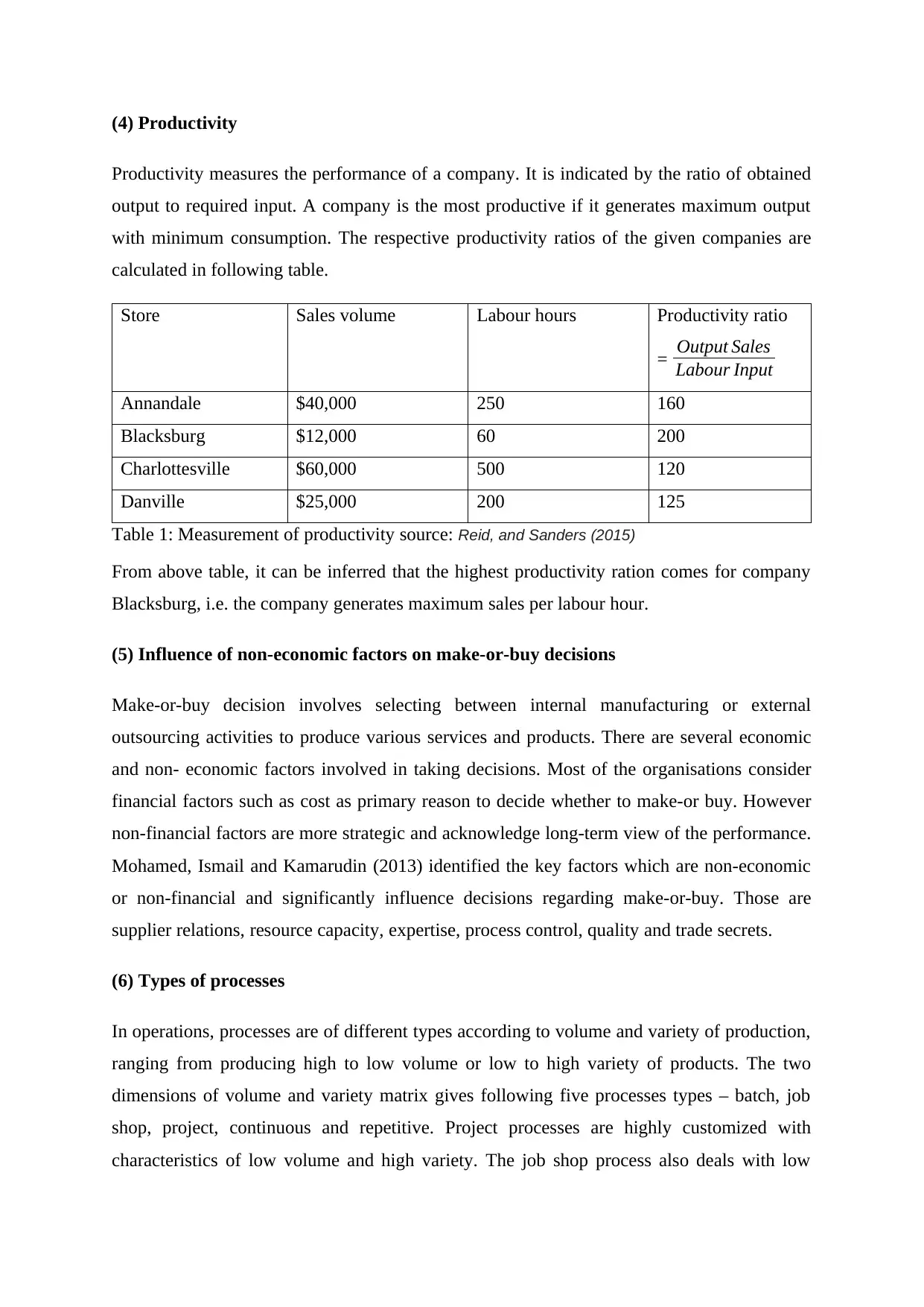
(4) Productivity
Productivity measures the performance of a company. It is indicated by the ratio of obtained
output to required input. A company is the most productive if it generates maximum output
with minimum consumption. The respective productivity ratios of the given companies are
calculated in following table.
Store Sales volume Labour hours Productivity ratio
= Output Sales
Labour Input
Annandale $40,000 250 160
Blacksburg $12,000 60 200
Charlottesville $60,000 500 120
Danville $25,000 200 125
Table 1: Measurement of productivity source: Reid, and Sanders (2015)
From above table, it can be inferred that the highest productivity ration comes for company
Blacksburg, i.e. the company generates maximum sales per labour hour.
(5) Influence of non-economic factors on make-or-buy decisions
Make-or-buy decision involves selecting between internal manufacturing or external
outsourcing activities to produce various services and products. There are several economic
and non- economic factors involved in taking decisions. Most of the organisations consider
financial factors such as cost as primary reason to decide whether to make-or buy. However
non-financial factors are more strategic and acknowledge long-term view of the performance.
Mohamed, Ismail and Kamarudin (2013) identified the key factors which are non-economic
or non-financial and significantly influence decisions regarding make-or-buy. Those are
supplier relations, resource capacity, expertise, process control, quality and trade secrets.
(6) Types of processes
In operations, processes are of different types according to volume and variety of production,
ranging from producing high to low volume or low to high variety of products. The two
dimensions of volume and variety matrix gives following five processes types – batch, job
shop, project, continuous and repetitive. Project processes are highly customized with
characteristics of low volume and high variety. The job shop process also deals with low
volume and high variety but produce physically smaller products and have fewer volatile
situations than project. Thus, it can be said that project processes are much complex than job
processes. Batch processes have moderately higher volume than project and job shop but
have lower degree of varieties. Repetitive processes are mass processes which produce
relatively higher volume with narrow degree of variety. Continuous processes are further one
step ahead of repetitive process that produce much higher volume with even lower variety
(Mahadevan, 2015).
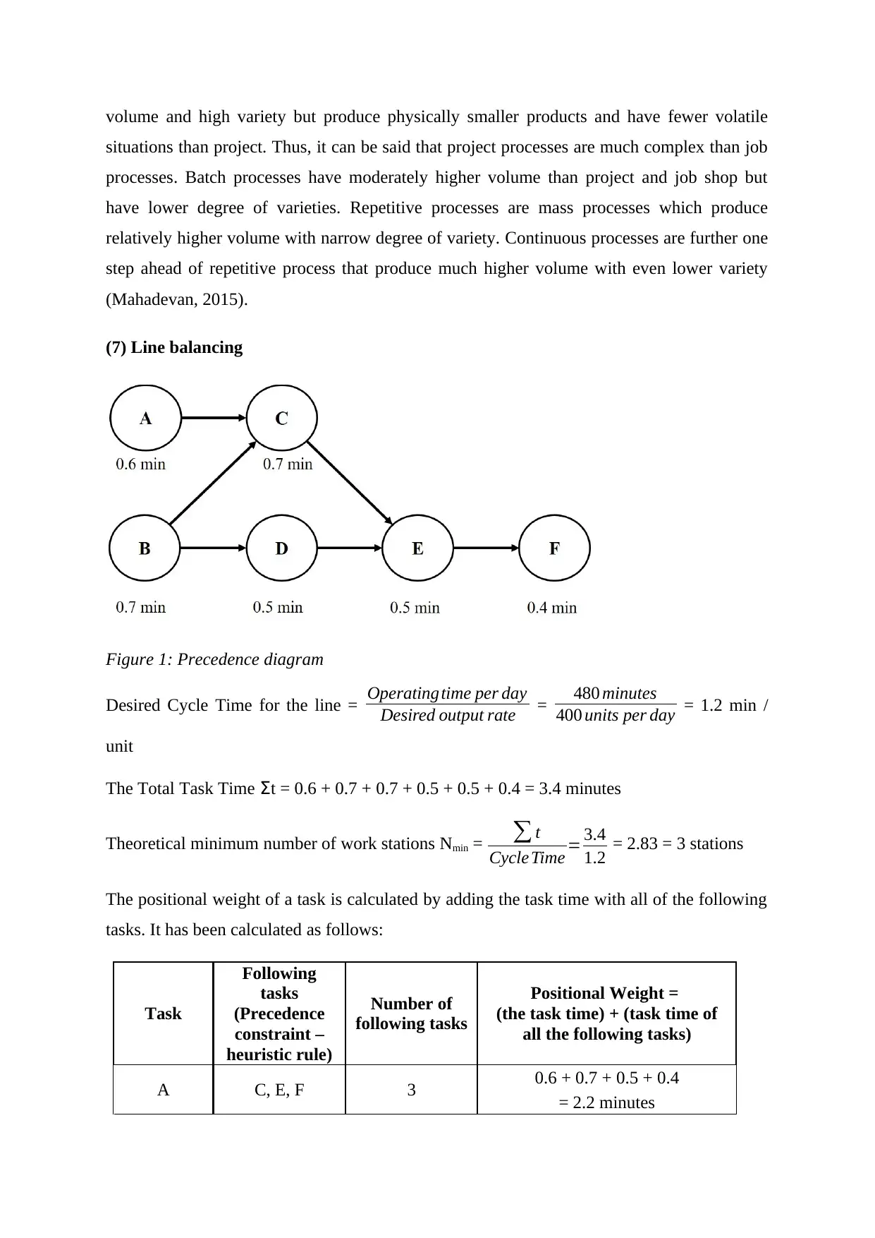
(7) Line balancing
Figure 1: Precedence diagram
Desired Cycle Time for the line = Operatingtime per day
Desired output rate = 480 minutes
400 units per day = 1.2 min /
unit
The Total Task Time Σt = 0.6 + 0.7 + 0.7 + 0.5 + 0.5 + 0.4 = 3.4 minutes
Theoretical minimum number of work stations Nmin = ∑ t
Cycle Time = 3.4
1.2 = 2.83 = 3 stations
The positional weight of a task is calculated by adding the task time with all of the following
tasks. It has been calculated as follows:
Task
Following
tasks
(Precedence
constraint –
heuristic rule)
Number of
following tasks
Positional Weight =
(the task time) + (task time of
all the following tasks)
A C, E, F 3 0.6 + 0.7 + 0.5 + 0.4
= 2.2 minutes
situations than project. Thus, it can be said that project processes are much complex than job
processes. Batch processes have moderately higher volume than project and job shop but
have lower degree of varieties. Repetitive processes are mass processes which produce
relatively higher volume with narrow degree of variety. Continuous processes are further one
step ahead of repetitive process that produce much higher volume with even lower variety
(Mahadevan, 2015).
(7) Line balancing
Figure 1: Precedence diagram
Desired Cycle Time for the line = Operatingtime per day
Desired output rate = 480 minutes
400 units per day = 1.2 min /
unit
The Total Task Time Σt = 0.6 + 0.7 + 0.7 + 0.5 + 0.5 + 0.4 = 3.4 minutes
Theoretical minimum number of work stations Nmin = ∑ t
Cycle Time = 3.4
1.2 = 2.83 = 3 stations
The positional weight of a task is calculated by adding the task time with all of the following
tasks. It has been calculated as follows:
Task
Following
tasks
(Precedence
constraint –
heuristic rule)
Number of
following tasks
Positional Weight =
(the task time) + (task time of
all the following tasks)
A C, E, F 3 0.6 + 0.7 + 0.5 + 0.4
= 2.2 minutes
⊘ This is a preview!⊘
Do you want full access?
Subscribe today to unlock all pages.
Trusted by 1+ million students worldwide
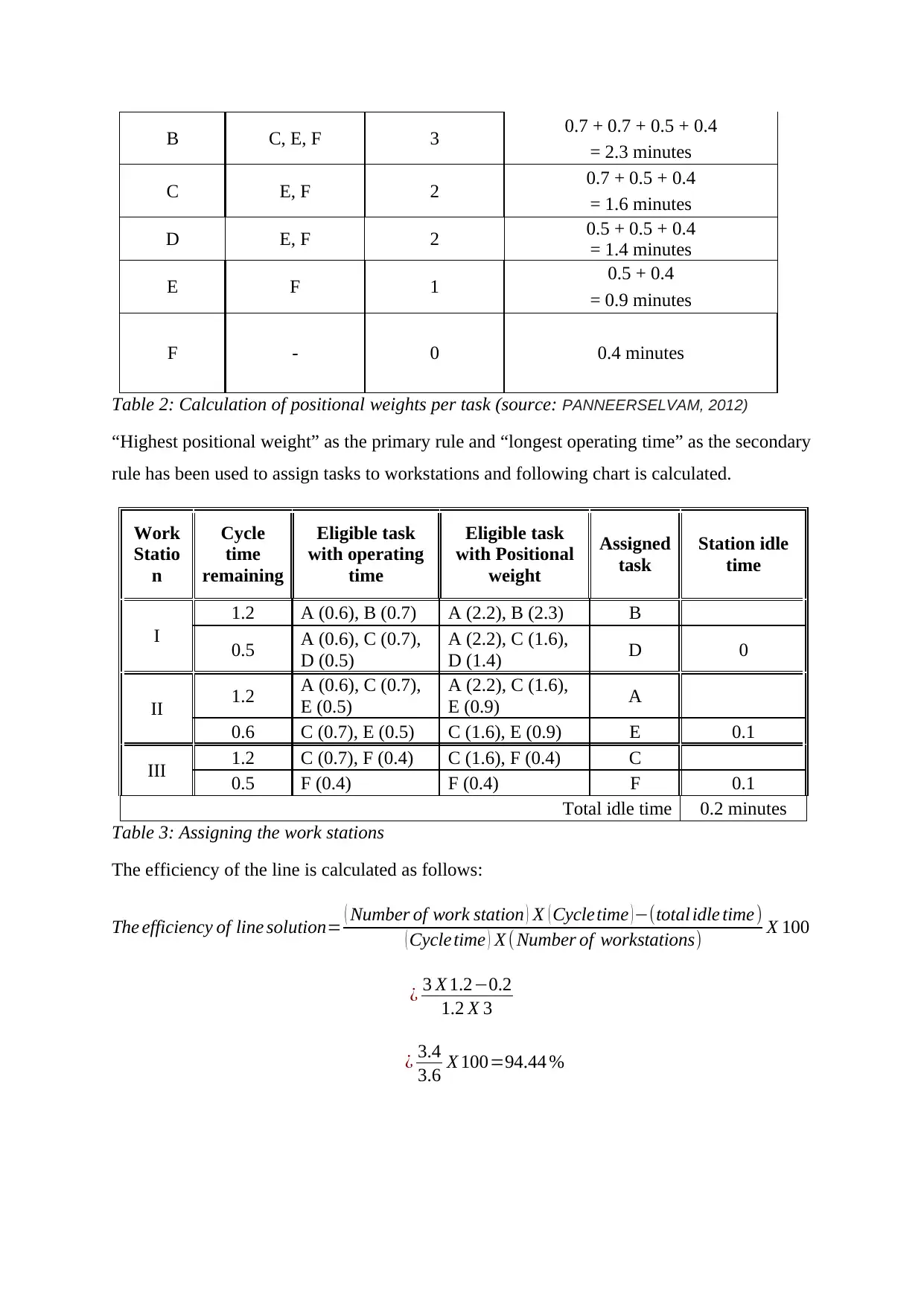
B C, E, F 3 0.7 + 0.7 + 0.5 + 0.4
= 2.3 minutes
C E, F 2 0.7 + 0.5 + 0.4
= 1.6 minutes
D E, F 2 0.5 + 0.5 + 0.4
= 1.4 minutes
E F 1 0.5 + 0.4
= 0.9 minutes
F - 0 0.4 minutes
Table 2: Calculation of positional weights per task (source: PANNEERSELVAM, 2012)
“Highest positional weight” as the primary rule and “longest operating time” as the secondary
rule has been used to assign tasks to workstations and following chart is calculated.
Work
Statio
n
Cycle
time
remaining
Eligible task
with operating
time
Eligible task
with Positional
weight
Assigned
task
Station idle
time
I
1.2 A (0.6), B (0.7) A (2.2), B (2.3) B
0.5 A (0.6), C (0.7),
D (0.5)
A (2.2), C (1.6),
D (1.4) D 0
II 1.2 A (0.6), C (0.7),
E (0.5)
A (2.2), C (1.6),
E (0.9) A
0.6 C (0.7), E (0.5) C (1.6), E (0.9) E 0.1
III 1.2 C (0.7), F (0.4) C (1.6), F (0.4) C
0.5 F (0.4) F (0.4) F 0.1
Total idle time 0.2 minutes
Table 3: Assigning the work stations
The efficiency of the line is calculated as follows:
The efficiency of line solution= ( Number of work station ) X ( Cycletime )−(total idle time)
( Cycle time ) X ( Number of workstations) X 100
¿ 3 X 1.2−0.2
1.2 X 3
¿ 3.4
3.6 X 100=94.44 %
Paraphrase This Document
Need a fresh take? Get an instant paraphrase of this document with our AI Paraphraser
(8) Job design and methods analysis
The main difference between job design and method analysis is that former is more of a
generic term which specifies the structure of working environment and main job contents,
whereas, method analysis is systematic approach which determines how the activities will be
carried out in order to perform a job.
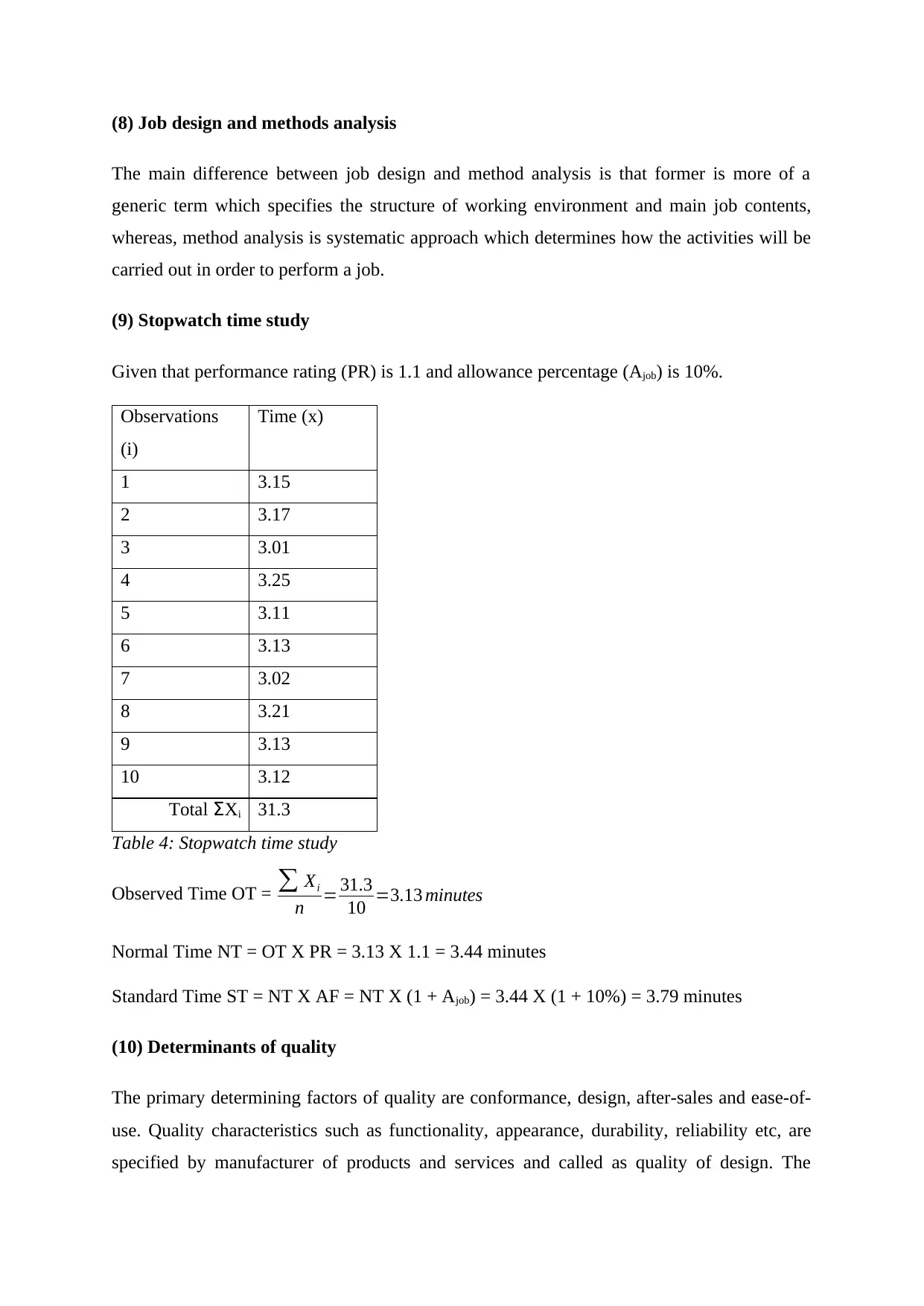
(9) Stopwatch time study
Given that performance rating (PR) is 1.1 and allowance percentage (Ajob) is 10%.
Observations
(i)
Time (x)
1 3.15
2 3.17
3 3.01
4 3.25
5 3.11
6 3.13
7 3.02
8 3.21
9 3.13
10 3.12
Total ΣXi 31.3
Table 4: Stopwatch time study
Observed Time OT = ∑ Xi
n = 31.3
10 =3.13 minutes
Normal Time NT = OT X PR = 3.13 X 1.1 = 3.44 minutes
Standard Time ST = NT X AF = NT X (1 + Ajob) = 3.44 X (1 + 10%) = 3.79 minutes
(10) Determinants of quality
The primary determining factors of quality are conformance, design, after-sales and ease-of-
use. Quality characteristics such as functionality, appearance, durability, reliability etc, are
specified by manufacturer of products and services and called as quality of design. The
The main difference between job design and method analysis is that former is more of a
generic term which specifies the structure of working environment and main job contents,
whereas, method analysis is systematic approach which determines how the activities will be
carried out in order to perform a job.
(9) Stopwatch time study
Given that performance rating (PR) is 1.1 and allowance percentage (Ajob) is 10%.
Observations
(i)
Time (x)
1 3.15
2 3.17
3 3.01
4 3.25
5 3.11
6 3.13
7 3.02
8 3.21
9 3.13
10 3.12
Total ΣXi 31.3
Table 4: Stopwatch time study
Observed Time OT = ∑ Xi
n = 31.3
10 =3.13 minutes
Normal Time NT = OT X PR = 3.13 X 1.1 = 3.44 minutes
Standard Time ST = NT X AF = NT X (1 + Ajob) = 3.44 X (1 + 10%) = 3.79 minutes
(10) Determinants of quality
The primary determining factors of quality are conformance, design, after-sales and ease-of-
use. Quality characteristics such as functionality, appearance, durability, reliability etc, are
specified by manufacturer of products and services and called as quality of design. The
internal quality specification when matched with the actual quality of product and services, it
provides quality of conformance. When customers’ own perception of quality is matched
with the actual quality of products, it determines ease-of-use. The after-sales service also
determines the perceived quality of products which arrives from organisations’ efforts of
taking care of issues after the sales.
(11) Costs of quality
The quality costs are either investment cost for good quality or overheads due to poor quality.
It comprises of three major costs of quality – failure, prevention and appraisal costs. The
appraisal costs include costs related to assessment and examination of materials and
equipment, costs of testing quality characteristics of finished products and various other
operating costs to maintain standard quality. Prevention costs involve costs of product design,
developing and implementing quality standards, training, and acquiring and analysing
information related to quality. Failure costs are of two types external and internal. Internal
failure costs are sustained in solving issues that are noticed before product delivery to
customers such as scrap cost, rework cost, price downgrading costs, process failure and
downtime costs. On the other hand, external failure costs are detected after the product
deliver to customers such as warranty claims, product returns, lost sales costs and other
complaints costs (Wudhikarn, 2012).
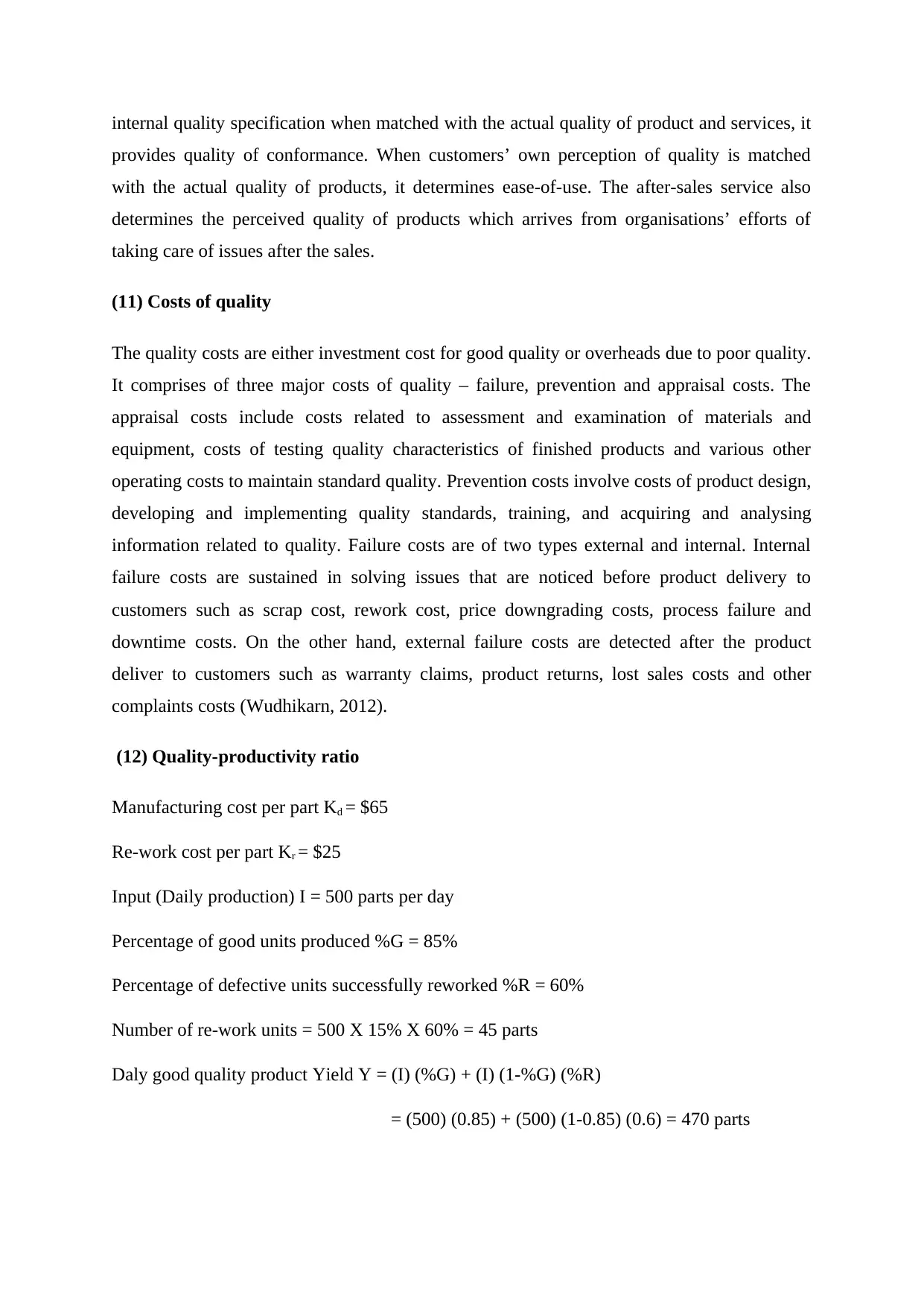
(12) Quality-productivity ratio
Manufacturing cost per part Kd = $65
Re-work cost per part Kr = $25
Input (Daily production) I = 500 parts per day
Percentage of good units produced %G = 85%
Percentage of defective units successfully reworked %R = 60%
Number of re-work units = 500 X 15% X 60% = 45 parts
Daly good quality product Yield Y = (I) (%G) + (I) (1-%G) (%R)
= (500) (0.85) + (500) (1-0.85) (0.6) = 470 parts
provides quality of conformance. When customers’ own perception of quality is matched
with the actual quality of products, it determines ease-of-use. The after-sales service also
determines the perceived quality of products which arrives from organisations’ efforts of
taking care of issues after the sales.
(11) Costs of quality
The quality costs are either investment cost for good quality or overheads due to poor quality.
It comprises of three major costs of quality – failure, prevention and appraisal costs. The
appraisal costs include costs related to assessment and examination of materials and
equipment, costs of testing quality characteristics of finished products and various other
operating costs to maintain standard quality. Prevention costs involve costs of product design,
developing and implementing quality standards, training, and acquiring and analysing
information related to quality. Failure costs are of two types external and internal. Internal
failure costs are sustained in solving issues that are noticed before product delivery to
customers such as scrap cost, rework cost, price downgrading costs, process failure and
downtime costs. On the other hand, external failure costs are detected after the product
deliver to customers such as warranty claims, product returns, lost sales costs and other
complaints costs (Wudhikarn, 2012).
(12) Quality-productivity ratio
Manufacturing cost per part Kd = $65
Re-work cost per part Kr = $25
Input (Daily production) I = 500 parts per day
Percentage of good units produced %G = 85%
Percentage of defective units successfully reworked %R = 60%
Number of re-work units = 500 X 15% X 60% = 45 parts
Daly good quality product Yield Y = (I) (%G) + (I) (1-%G) (%R)
= (500) (0.85) + (500) (1-0.85) (0.6) = 470 parts
⊘ This is a preview!⊘
Do you want full access?
Subscribe today to unlock all pages.
Trusted by 1+ million students worldwide
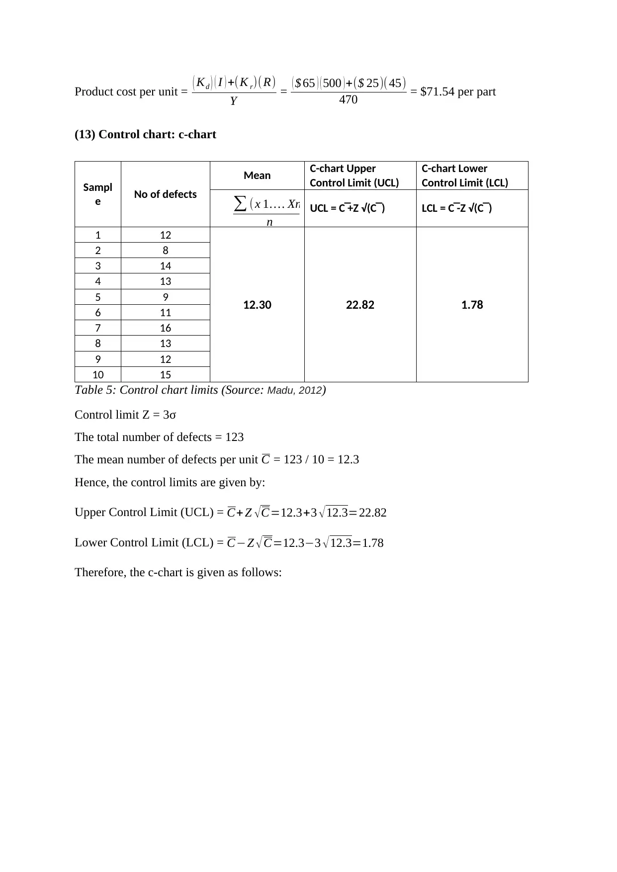
Product cost per unit = ( Kd ) ( I ) +(K r)( R)
Y = ( $ 65 ) ( 500 )+($ 25)(45)
470 = $71.54 per part
(13) Control chart: c-chart
Sampl
e No of defects
Mean C-chart Upper
Control Limit (UCL)
C-chart Lower
Control Limit (LCL)
UCL = C ̅ +Z √(C ̅ ) LCL = C ̅ -Z √(C ̅ )
1 12
12.30 22.82 1.78
2 8
3 14
4 13
5 9
6 11
7 16
8 13
9 12
10 15
Table 5: Control chart limits (Source: Madu, 2012)
Control limit Z = 3σ
The total number of defects = 123
The mean number of defects per unit C = 123 / 10 = 12.3
Hence, the control limits are given by:
Upper Control Limit (UCL) = C+ Z √C=12.3+3 √12.3=22.82
Lower Control Limit (LCL) = C−Z √ C=12.3−3 √12.3=1.78
Therefore, the c-chart is given as follows:
∑ ( x 1… . Xn)
n
Paraphrase This Document
Need a fresh take? Get an instant paraphrase of this document with our AI Paraphraser
0
5
10
15
20
25
1 2 3 4 5 6 7 8 9 10
Number of defects
Sample
C-Chart
No of defects
Mean
C-chart Upper Control Limit
(UCL)
C-chart Lower Control Limit
(LCL)
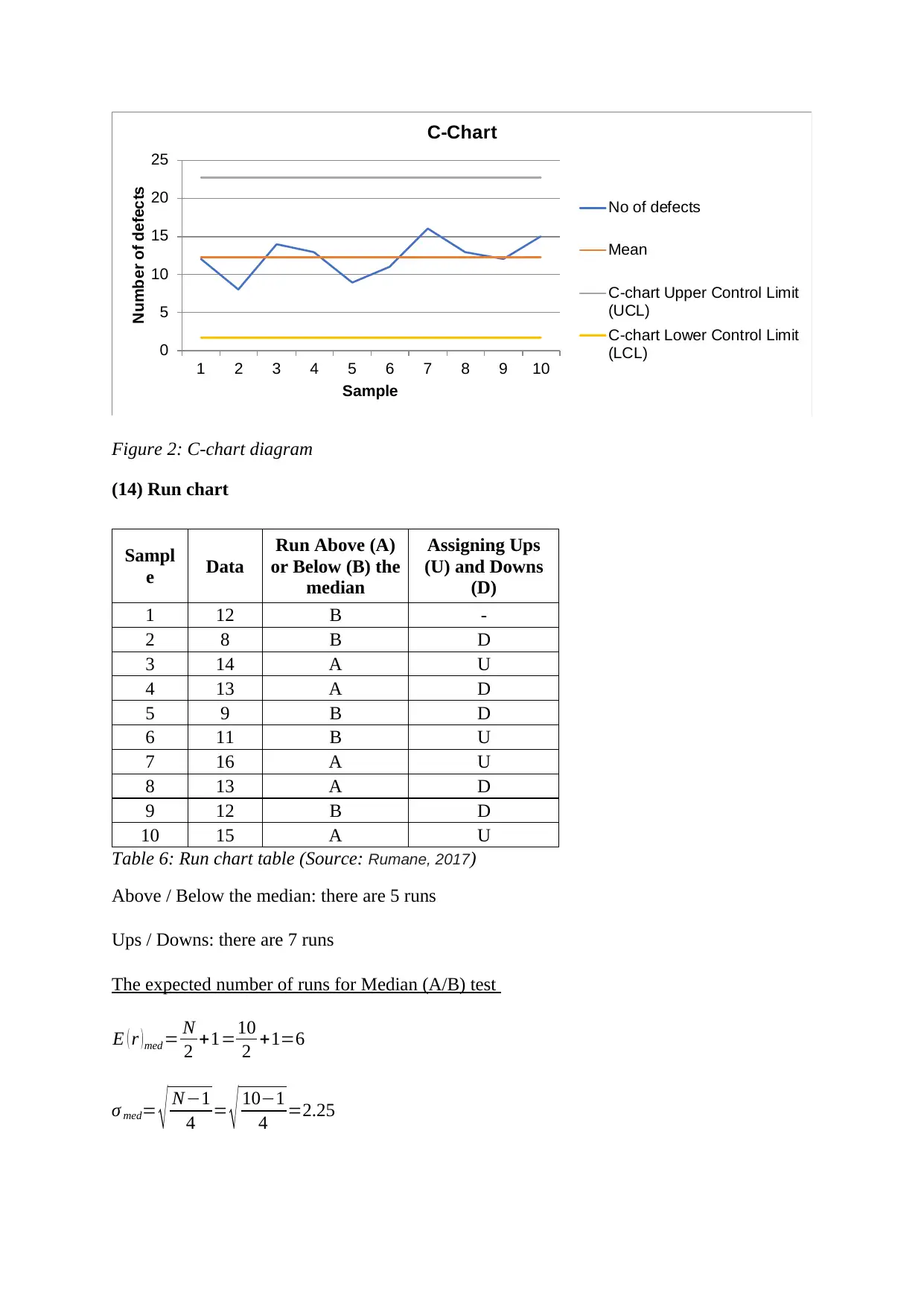
Figure 2: C-chart diagram
(14) Run chart
Sampl
e Data
Run Above (A)
or Below (B) the
median
Assigning Ups
(U) and Downs
(D)
1 12 B -
2 8 B D
3 14 A U
4 13 A D
5 9 B D
6 11 B U
7 16 A U
8 13 A D
9 12 B D
10 15 A U
Table 6: Run chart table (Source: Rumane, 2017)
Above / Below the median: there are 5 runs
Ups / Downs: there are 7 runs
The expected number of runs for Median (A/B) test
E ( r )med = N
2 +1=10
2 +1=6
σ med= √ N−1
4 = √ 10−1
4 =2.25
5
10
15
20
25
1 2 3 4 5 6 7 8 9 10
Number of defects
Sample
C-Chart
No of defects
Mean
C-chart Upper Control Limit
(UCL)
C-chart Lower Control Limit
(LCL)
Figure 2: C-chart diagram
(14) Run chart
Sampl
e Data
Run Above (A)
or Below (B) the
median
Assigning Ups
(U) and Downs
(D)
1 12 B -
2 8 B D
3 14 A U
4 13 A D
5 9 B D
6 11 B U
7 16 A U
8 13 A D
9 12 B D
10 15 A U
Table 6: Run chart table (Source: Rumane, 2017)
Above / Below the median: there are 5 runs
Ups / Downs: there are 7 runs
The expected number of runs for Median (A/B) test
E ( r )med = N
2 +1=10
2 +1=6
σ med= √ N−1
4 = √ 10−1
4 =2.25
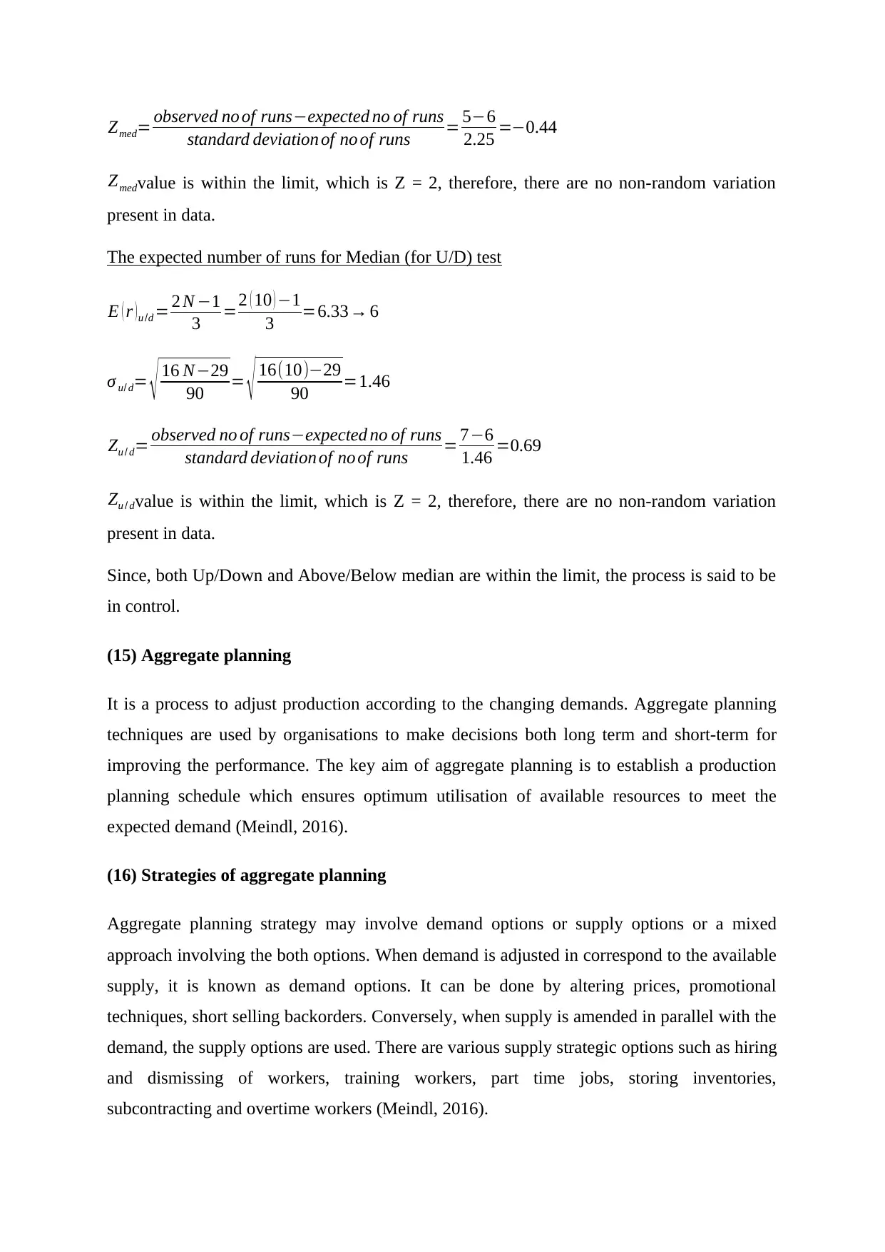
Zmed= observed no of runs−expected no of runs
standard deviation of no of runs = 5−6
2.25 =−0.44
Zmedvalue is within the limit, which is Z = 2, therefore, there are no non-random variation
present in data.
The expected number of runs for Median (for U/D) test
E ( r )u /d = 2 N −1
3 =2 ( 10 ) −1
3 =6.33→ 6
σ u/ d= √ 16 N−29
90 = √ 16(10)−29
90 =1.46
Zu / d= observed no of runs−expected no of runs
standard deviation of no of runs = 7−6
1.46 =0.69
Zu / dvalue is within the limit, which is Z = 2, therefore, there are no non-random variation
present in data.
Since, both Up/Down and Above/Below median are within the limit, the process is said to be
in control.
(15) Aggregate planning
It is a process to adjust production according to the changing demands. Aggregate planning
techniques are used by organisations to make decisions both long term and short-term for
improving the performance. The key aim of aggregate planning is to establish a production
planning schedule which ensures optimum utilisation of available resources to meet the
expected demand (Meindl, 2016).
(16) Strategies of aggregate planning
Aggregate planning strategy may involve demand options or supply options or a mixed
approach involving the both options. When demand is adjusted in correspond to the available
supply, it is known as demand options. It can be done by altering prices, promotional
techniques, short selling backorders. Conversely, when supply is amended in parallel with the
demand, the supply options are used. There are various supply strategic options such as hiring
and dismissing of workers, training workers, part time jobs, storing inventories,
subcontracting and overtime workers (Meindl, 2016).
⊘ This is a preview!⊘
Do you want full access?
Subscribe today to unlock all pages.
Trusted by 1+ million students worldwide
1 out of 19
Related Documents


Your All-in-One AI-Powered Toolkit for Academic Success.
+13062052269
info@desklib.com
Available 24*7 on WhatsApp / Email
![[object Object]](/_next/static/media/star-bottom.7253800d.svg)
Unlock your academic potential
Copyright © 2020–2026 A2Z Services. All Rights Reserved. Developed and managed by ZUCOL.