Operations Research Assignment: Linear Programming, Network, and EOQ

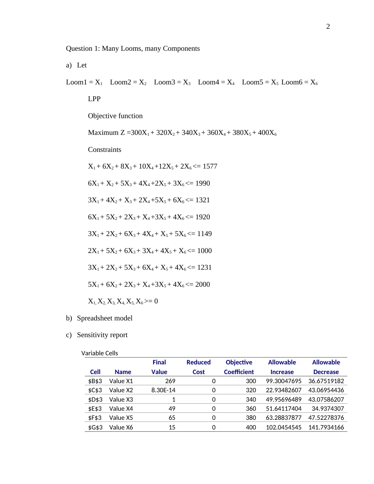
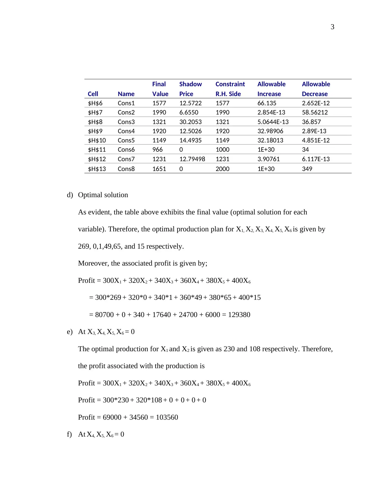
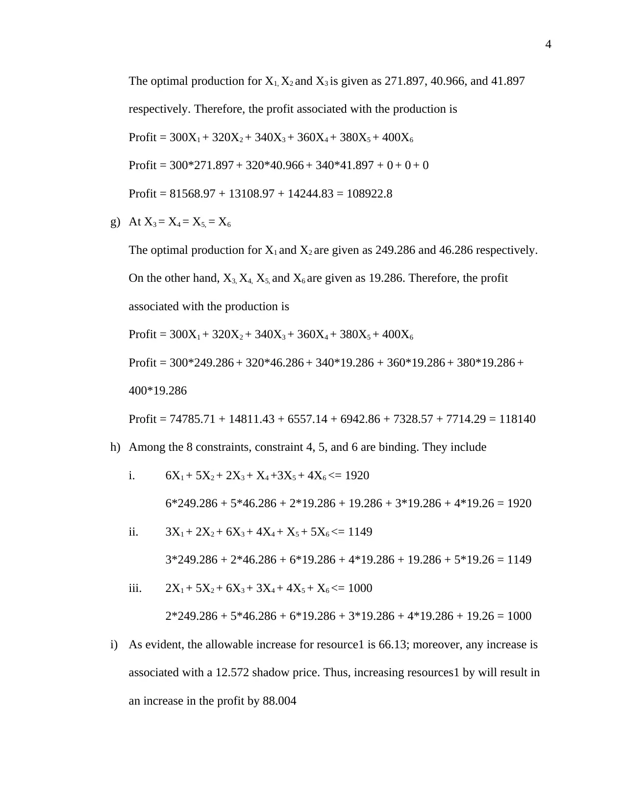
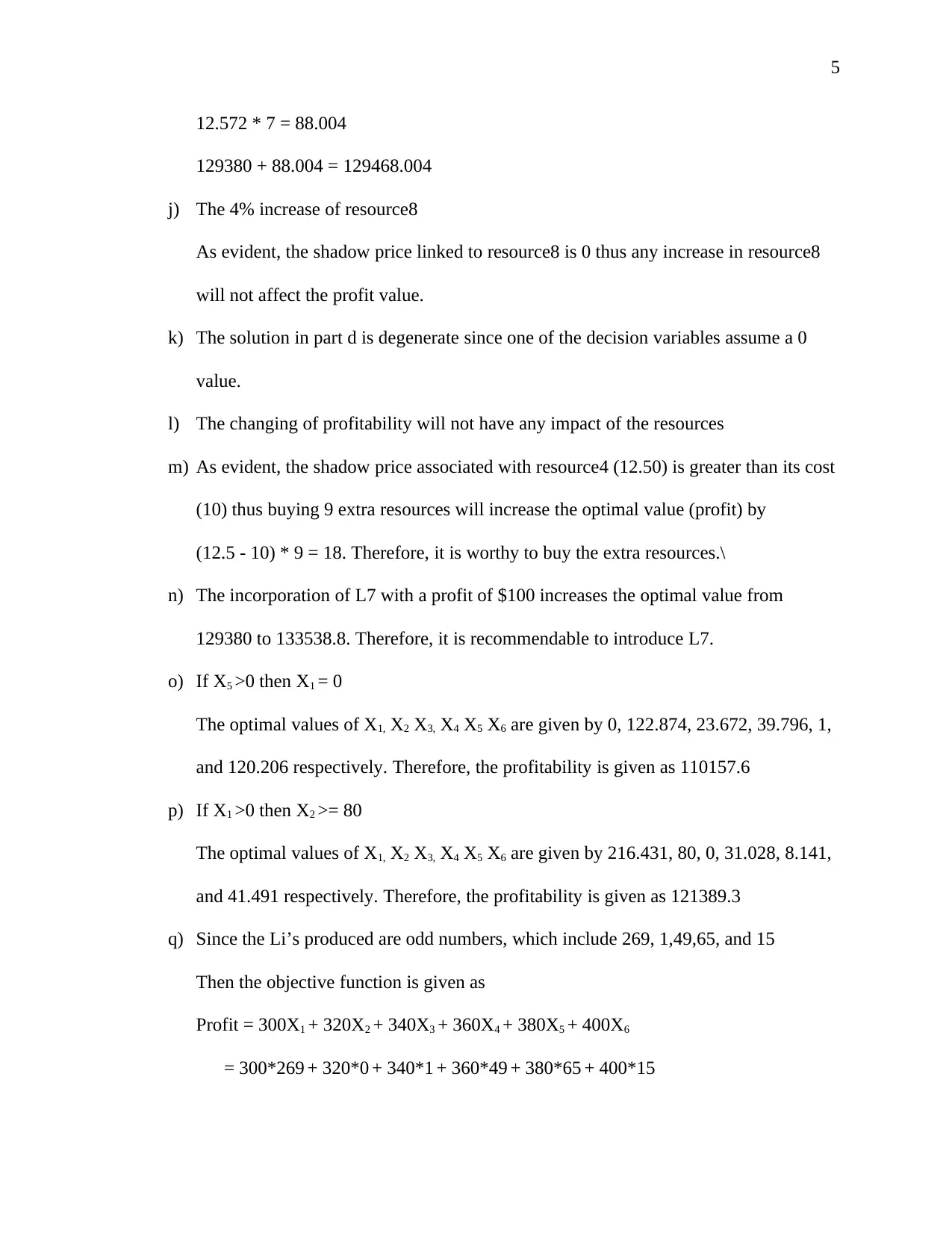
This document presents a comprehensive solution to an Operations Research assignment, encompassing three key areas: linear programming, network transshipment, and Economic Order Quantity (EOQ) inventory management. The linear programming section involves optimizing production plans for multiple looms, utilizing Excel Solver to determine the optimal values for each loom and calculating the associated profit. Sensitivity analysis is conducted to evaluate the impact of changes in resources and profitability. The network transshipment problem focuses on minimizing the cost of transporting goods between various locations, with the solution including optimal flow routes and associated costs. Finally, the EOQ section addresses inventory management, calculating the optimal order quantity and related costs. The solution provides detailed steps, calculations, and interpretations of the results, including the use of Excel Solver and sensitivity reports.

1
Operation Research
Name:
Institution:

2
Question 1: Many Looms, many Components
a) Let
Loom1 = X1 Loom2 = X2 Loom3 = X3 Loom4 = X4 Loom5 = X5 Loom6 = X6
LPP
Objective function
Maximum Z =300X1 + 320X2 + 340X3 + 360X4 + 380X5 + 400X6
Constraints
X1 + 6X2 + 8X3 + 10X4 +12X5 + 2X6 <= 1577
6X1 + X2 + 5X3 + 4X4 +2X5 + 3X6 <= 1990
3X1 + 4X2 + X3 + 2X4 +5X5 + 6X6 <= 1321
6X1 + 5X2 + 2X3 + X4 +3X5 + 4X6 <= 1920
3X1 + 2X2 + 6X3 + 4X4 + X5 + 5X6 <= 1149
2X1 + 5X2 + 6X3 + 3X4 + 4X5 + X6 <= 1000
3X1 + 2X2 + 5X3 + 6X4 + X5 + 4X6 <= 1231
5X1 + 6X2 + 2X3 + X4 +3X5 + 4X6 <= 2000
X1, X2, X3, X4, X5, X6 >= 0
b) Spreadsheet model
c) Sensitivity report
Variable Cells
Final Reduced Objective Allowable Allowable
Cell Name Value Cost Coefficient Increase Decrease
$B$3 Value X1 269 0 300 99.30047695 36.67519182
$C$3 Value X2 8.30E-14 0 320 22.93482607 43.06954436
$D$3 Value X3 1 0 340 49.95696489 43.07586207
$E$3 Value X4 49 0 360 51.64117404 34.9374307
$F$3 Value X5 65 0 380 63.28837877 47.52278376
$G$3 Value X6 15 0 400 102.0454545 141.7934166

3
Final Shadow Constraint Allowable Allowable
Cell Name Value Price R.H. Side Increase Decrease
$H$6 Cons1 1577 12.5722 1577 66.135 2.652E-12
$H$7 Cons2 1990 6.6550 1990 2.854E-13 58.56212
$H$8 Cons3 1321 30.2053 1321 5.0644E-13 36.857
$H$9 Cons4 1920 12.5026 1920 32.98906 2.89E-13
$H$10 Cons5 1149 14.4935 1149 32.18013 4.851E-12
$H$11 Cons6 966 0 1000 1E+30 34
$H$12 Cons7 1231 12.79498 1231 3.90761 6.117E-13
$H$13 Cons8 1651 0 2000 1E+30 349
d) Optimal solution
As evident, the table above exhibits the final value (optimal solution for each
variable). Therefore, the optimal production plan for X1, X2, X3, X4, X5, X6 is given by
269, 0,1,49,65, and 15 respectively.
Moreover, the associated profit is given by;
Profit = 300X1 + 320X2 + 340X3 + 360X4 + 380X5 + 400X6
= 300*269 + 320*0 + 340*1 + 360*49 + 380*65 + 400*15
= 80700 + 0 + 340 + 17640 + 24700 + 6000 = 129380
e) At X3, X4, X5, X6 = 0
The optimal production for X1 and X2 is given as 230 and 108 respectively. Therefore,
the profit associated with the production is
Profit = 300X1 + 320X2 + 340X3 + 360X4 + 380X5 + 400X6
Profit = 300*230 + 320*108 + 0 + 0 + 0 + 0
Profit = 69000 + 34560 = 103560
f) At X4, X5, X6 = 0

4
The optimal production for X1, X2 and X3 is given as 271.897, 40.966, and 41.897
respectively. Therefore, the profit associated with the production is
Profit = 300X1 + 320X2 + 340X3 + 360X4 + 380X5 + 400X6
Profit = 300*271.897 + 320*40.966 + 340*41.897 + 0 + 0 + 0
Profit = 81568.97 + 13108.97 + 14244.83 = 108922.8
g) At X3 = X4 = X5, = X6
The optimal production for X1 and X2 are given as 249.286 and 46.286 respectively.
On the other hand, X3, X4, X5, and X6 are given as 19.286. Therefore, the profit
associated with the production is
Profit = 300X1 + 320X2 + 340X3 + 360X4 + 380X5 + 400X6
Profit = 300*249.286 + 320*46.286 + 340*19.286 + 360*19.286 + 380*19.286 +
400*19.286
Profit = 74785.71 + 14811.43 + 6557.14 + 6942.86 + 7328.57 + 7714.29 = 118140
h) Among the 8 constraints, constraint 4, 5, and 6 are binding. They include
i. 6X1 + 5X2 + 2X3 + X4 +3X5 + 4X6 <= 1920
6*249.286 + 5*46.286 + 2*19.286 + 19.286 + 3*19.286 + 4*19.26 = 1920
ii. 3X1 + 2X2 + 6X3 + 4X4 + X5 + 5X6 <= 1149
3*249.286 + 2*46.286 + 6*19.286 + 4*19.286 + 19.286 + 5*19.26 = 1149
iii. 2X1 + 5X2 + 6X3 + 3X4 + 4X5 + X6 <= 1000
2*249.286 + 5*46.286 + 6*19.286 + 3*19.286 + 4*19.286 + 19.26 = 1000
i) As evident, the allowable increase for resource1 is 66.13; moreover, any increase is
associated with a 12.572 shadow price. Thus, increasing resources1 by will result in
an increase in the profit by 88.004

5
12.572 * 7 = 88.004
129380 + 88.004 = 129468.004
j) The 4% increase of resource8
As evident, the shadow price linked to resource8 is 0 thus any increase in resource8
will not affect the profit value.
k) The solution in part d is degenerate since one of the decision variables assume a 0
value.
l) The changing of profitability will not have any impact of the resources
m) As evident, the shadow price associated with resource4 (12.50) is greater than its cost
(10) thus buying 9 extra resources will increase the optimal value (profit) by
(12.5 - 10) * 9 = 18. Therefore, it is worthy to buy the extra resources.\
n) The incorporation of L7 with a profit of $100 increases the optimal value from
129380 to 133538.8. Therefore, it is recommendable to introduce L7.
o) If X5 >0 then X1 = 0
The optimal values of X1, X2 X3, X4 X5 X6 are given by 0, 122.874, 23.672, 39.796, 1,
and 120.206 respectively. Therefore, the profitability is given as 110157.6
p) If X1 >0 then X2 >= 80
The optimal values of X1, X2 X3, X4 X5 X6 are given by 216.431, 80, 0, 31.028, 8.141,
and 41.491 respectively. Therefore, the profitability is given as 121389.3
q) Since the Li’s produced are odd numbers, which include 269, 1,49,65, and 15
Then the objective function is given as
Profit = 300X1 + 320X2 + 340X3 + 360X4 + 380X5 + 400X6
= 300*269 + 320*0 + 340*1 + 360*49 + 380*65 + 400*15

6
= 80700 + 0 + 340 + 17640 + 24700 + 6000 = 129380
r) Since there are no even numbered Li’s produced, then objective function is given as
= 300*0 + 320*0 + 340*0 + 360*0 + 380*0 + 400*0
= 0
s) There are 5Li’s greater than 0 (Li>0)
Start-up cost = 2000 * 5 = 10,000
Objective = 129380 – 10,000
= 119380
t) Since there are no even numbered Li’s produced, then objective function is given as 0
Question 2 Network Transshipment
a) Let AG = Aldinga to Geelong
AK = Aldinga to Kalgoorlie
CG = Canberra to Geelong
CK = Canberra to Kalgoorlie
GM = Geelong to Mittagong
GW = Geelong to Wanga
KM = Kalgoorlie to Mittagong
KW = Kalgoorlie to Wanga
Objective function
Minimization Z = 2AG + 8AK + 7CG + 4CK + 2GM + 3GW + 3KM + 6KW
Notes
i. -AG - AK = -80
ii. -CG - CK = -90

7
iii. AG + CG – GM – GW = 0
iv. AK + CK – KM – KW = 0
v. GM + KM = 70
vi. GW + KW = 100
The optimal solution AG, CG, CK, GW, and KM which are given as 80, 90, 80,
70, and 20 respectively.
Cost = 2*80 + 0 + 7*20 + 4*70 + 0 + 3*100 + 3*70 + 0
= 1090
b) GM first 40 = $2, the rest $9
GW first 50 =$3, the rest $10
Cost = 2*80 + 7*20 + 4*70 + 3*50 + 10*50 + 3*70 = 1440
c) Non-zero flow tax $150
Cost = 1090
The adjoining towns that have a non-zero flow is CK thus the edge penalty is $150
Therefore, the cost = 1090 + 150 = $1240
d) Hybrid b and c
i. Cost at b = 1440
Edge penalty = 140
Total cost = 1440 + 140 = 1580
ii. Cost at b = 1440
Edge penalty = 160
Total cost = 1440 + 160 = 1600
iii. Cost at b = 1440

8
Edge penalty = 280
Total cost = 1440 + 280 = 1720
e) Additional node
-AG – KM >= 100
-AG – KM <= 120
The optimal solution AG, CK, GM, GW, KM, and KW which are given as 80, 90, 50,
30, 20, and 70 respectively.
Cost = 2*80 + 0 + 0 + 4*90 + 2*50 + 3*300 + 3*20 + 6*70
= 1190
Question 3 Economic Order Quantity (EOQ)
Volume = 1000 per month
Purchase Cost = $625
Ordering cost = $15
Annual Holding cost = 40% of 625
a) EOQ
Q∗¿ √ 2 SD
H
Holding cost (H) = 250
S = 15
D = 12,000
Q∗¿ √ 2∗15∗12000
250
= 37.947 ≈ 38
b) As evident, the EOQ = 39

9
Therefore, the number of orders per annum should be
12000/38 = 316.222 ≈ 316
c) EOQ with back-orders
Qb= √ 2 SD
H ∗
√ H +Cb
Cb
Cb = 250 * 4 = 1000
Qb=37.947 √ 250+ 1000
1000
37.947 * 1.1180 = 42.4264 ≈ 42