OPS/571 Operations Forecasting Report

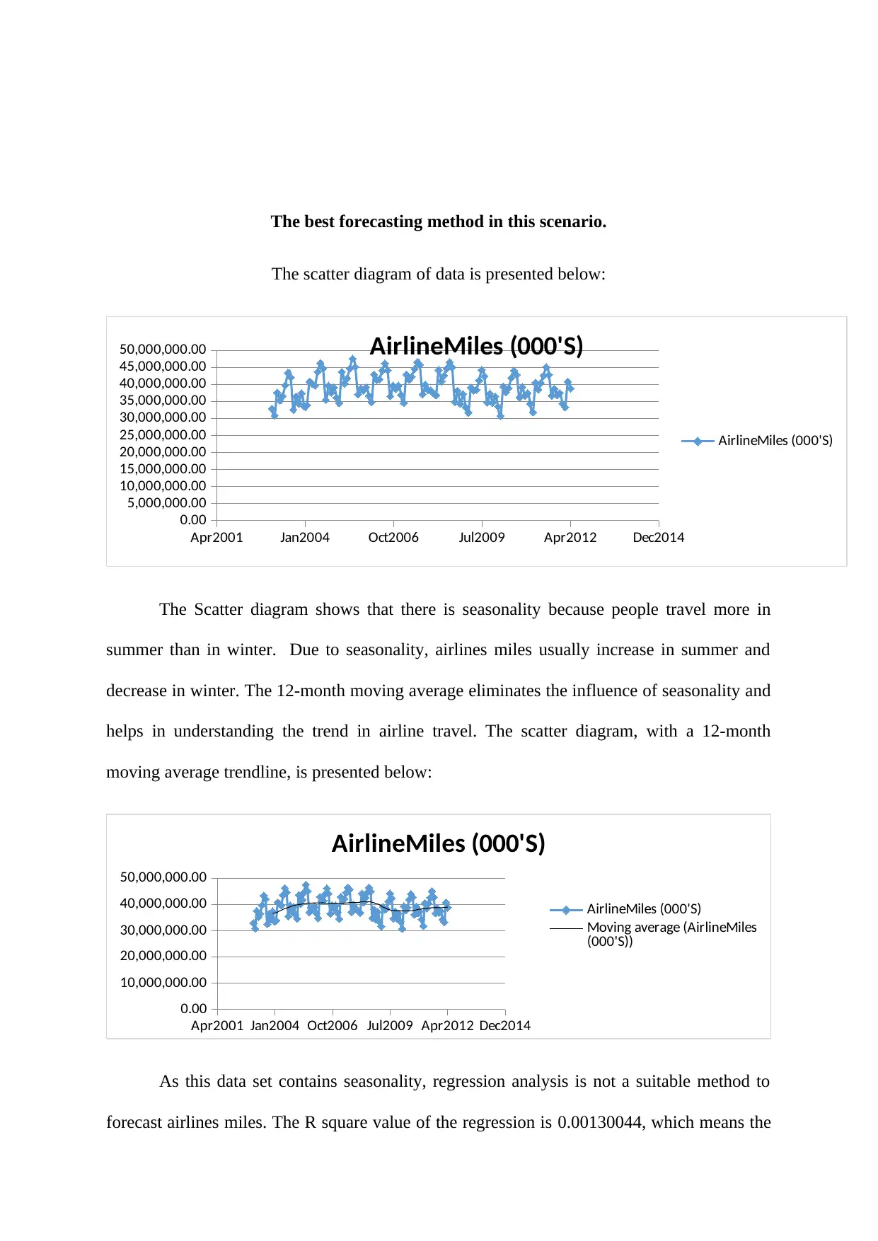
This report analyzes U.S. air passenger miles from 2003 to 2012, utilizing various forecasting models including time series, regression analysis, and seasonal models. It concludes that the additive model with trend and seasonality is the most effective for predicting airline miles, allowing companies to ...Read More

Operations Forecasting
Tamika D. Taylor
OPS/571
May 10, 2019
Sandra Norris

Introduction
The assignment has used the data of U.S. air passenger miles from 2003 to 2012. Various
forecasting models are used to forecast U.S. air passenger miles. This data set contains
monthly airlines miles (in thousands) travelled in the U.S. from January 2003 to April 2012.
Based on the given data, we had to forecast U.S. airlines miles in January 2013.
The forecasting models can be broadly categorized into three categories:
1. Time series models
2. Causal models
3. Qualitative models
Time series models
The time series models use historical data to forecast with the assumption that the future
is a function of the past. Some useful forecasting methods using historical data are
Regression Analysis, Moving Average, Exponential smoothing, Trend projection, etc. A time
series has three components: Trend (T), Seasonality (S), and Random variation (R).

Regression Analysis
Regression analysis can be used to forecast sales when there is a trend but no
seasonality or cycle. In regression analysis, the period is used as an independent variable.
Sales (dependent variable) is estimated as a function of period. (Winston, 2014) In Microsoft
Excel, regression analysis is conducted on given data using month number as independent
variable and monthly airlines miles as the dependent variable. Result of regression analysis is
presented below:
Regression Statistics
Multiple R 0.036061612
R Square 0.00130044
Adjusted R Square -0.007778647
Standard Error 3977747.757
Observations 112
Coefficients
Intercept 39355295.13
MonthNumber -4399.893724
A linear equation can be developed to forecast airline miles as:
Predicted airline miles = 39355295*period Number – 4400
Where airline miles is in thousands.
Now, to forecast U.S. airline miles in January 2013; first, we need to determine the period
number.

January 2013 is period number 121.
Thus, forecasted airlines miles in January 2013 = 39355295*121 – 4400 = 4761986295 (in
thousands)
Forecasted U.S. airlines miles in January 2013 = 4,761 billion
The R square value of this regression is 0.0013, which is very low. R square is the
power of regression. R square tells that this linear relationship explains 0.13% of the variation
in monthly U.S. airlines miles. The linear relationship obtained using regression analysis will
not predict the U.S. airlines miles correctly.
Additive Model with Trends and Seasonality
This model is useful when data has a trend and seasonality. In this model:
Predicted period t sales = Base + Trend*Period Number + Seasonality Index for month t
 The base is the best estimate of the level without seasonality at the beginning
of the period. The trend is the best estimate of the monthly rate of increase in
airline miles traveled. Each month of the year has a seasonal index. In
Microsoft Excel, Solver is used to determining base, trend, and seasonality
index for each month. (Winston, 2014) This model has RSQ value 0.989,
which means that this model explains that 98.9% of the variations in airline
miles traveled. In this case, the additive model is preferred over the
multiplicative model as the additive model has a lower standard deviation of
residuals.
Forecasted airlines miles traveled in January 2013 is 35.46 billion.

Multiplicative Model with Trend and Seasonality
The multiplicative model is used to estimate sales when data has trend and
seasonality. This is a non-linear forecasting model. In the multiplicative model:
Predicted period t sales = Base*Trend * Seasonal index for month t
In predictive model also, we need to estimate base, trend, and seasonal index. In
Microsoft Excel, Solver is used to determining base, trend, and seasonal index. (Winston,
2014) Using the multiplicative model, forecasted airlines miles traveled in January 2013 is
35.28 billion.
Comparison of Three Forecasting Methods
The regression analysis is useful when data does not contain seasonality. Regression
analysis is used when the data set has a trend only. Whether regression analysis is suitable to
forecast based on the given dataset or not can be determined from R square. R square is also
called the power of regression. High R square value indicates that the linear relationship
explains the number of deviations. When a data set has trend as well as seasonality, the
additive model with trend and seasonality, or multiplicative model with trend and seasonality
are more suitable. (Winston, 2014) The additive method is a linear forecasting method, while
the multiplicative method is nonlinear forecasting method. Between additive and
multiplicative method, a method having a lower standard deviation of residual is preferred.

The best forecasting method in this scenario.
The scatter diagram of data is presented below:
Apr2001 Jan2004 Oct2006 Jul2009 Apr2012 Dec2014
0.00
5,000,000.00
10,000,000.00
15,000,000.00
20,000,000.00
25,000,000.00
30,000,000.00
35,000,000.00
40,000,000.00
45,000,000.00
50,000,000.00 AirlineMiles (000'S)
AirlineMiles (000'S)
The Scatter diagram shows that there is seasonality because people travel more in
summer than in winter. Due to seasonality, airlines miles usually increase in summer and
decrease in winter. The 12-month moving average eliminates the influence of seasonality and
helps in understanding the trend in airline travel. The scatter diagram, with a 12-month
moving average trendline, is presented below:
Apr2001 Jan2004 Oct2006 Jul2009 Apr2012 Dec2014
0.00
10,000,000.00
20,000,000.00
30,000,000.00
40,000,000.00
50,000,000.00
AirlineMiles (000'S)
AirlineMiles (000'S)
Moving average (AirlineMiles
(000'S))
As this data set contains seasonality, regression analysis is not a suitable method to
forecast airlines miles. The R square value of the regression is 0.00130044, which means the

linear relationship obtained using regression analysis explains only 0.13% of the points.
When a data set has trend as well as seasonality, an additive model with trend and
seasonality, or multiplicative model with trend and seasonality are more suitable forecasting
methods. In this case, the standard deviation of residuals of the additive method is lower than
the standard deviation of residuals of the multiplicative method. Thus, the additive model
with trend and seasonality is the best for the firms. Using this method, an airline company can
predict the airlines' miles travelers will travel in a particular month. Based on this prediction,
an airlines company can plan a light schedule. The accuracy of the forecasting model will
help the airline company to plan flight schedules more confidently and achieve higher
occupancy rate. The forecasting of U.S. airlines miles will allow the airlines' companies to
run the optimal number of flights and save cost.
Time series analysis graph
Airline miles
0
10000000
20000000
30000000
40000000
50000000
60000000
Series1 Series2 Series3 Series4 Series5 Series6

References.
Winston, W. L., (2014). Marketing Analytics: Data-Driven Techniques with Microsoft Excel.
John Wiley & Sons, Inc.