Ordinary Least Squares Analysis Report - Intergenerational Education

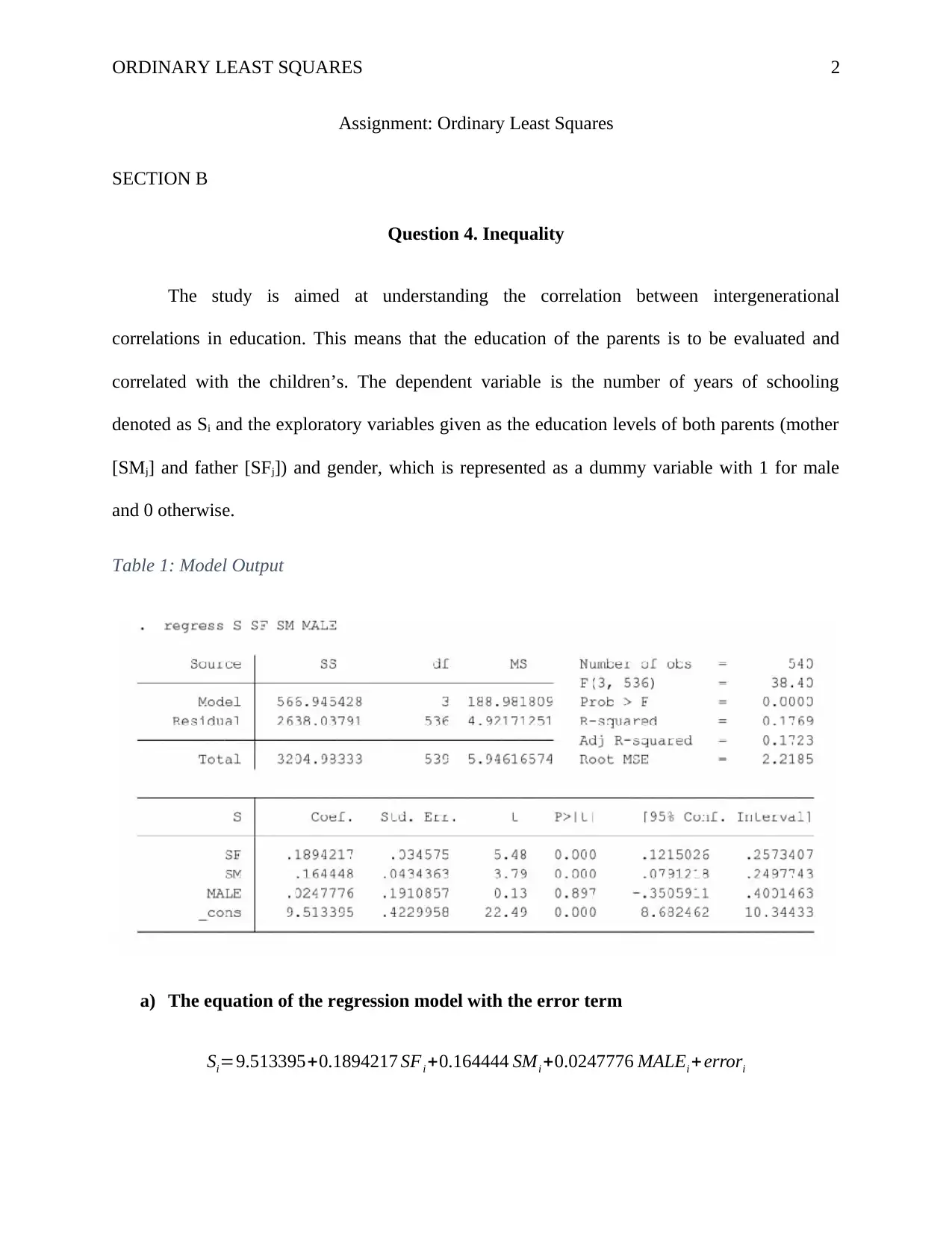
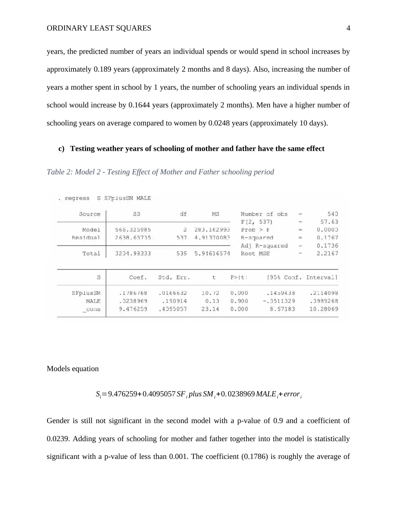
This report presents an Ordinary Least Squares (OLS) analysis focused on the correlation between intergenerational education. The study investigates how parents' education levels (mother and father) influence their children's years of schooling, using gender as a control variable. The analysis includes model output, coefficient interpretations, and hypothesis testing to determine statistical significance. The report examines the effects of each parent's education on their children's schooling, finding that both mother's and father's education significantly predict the number of years a child spends in school. The report also tests if the years of schooling of the mother and father have the same effect on the child's schooling years. The report concludes with a discussion of the assumptions of OLS regression. The findings indicate that the model is statistically significant, with parents' education having a positive impact on their children's education. Furthermore, the study highlights the importance of understanding intergenerational educational correlations for informed decision-making.

Running head: ORDINARY LEAST SQUARES
Assignment: Ordinary Least Squares
Name
Course Number
Date
Faculty Name

ORDINARY LEAST SQUARES 2
Assignment: Ordinary Least Squares
SECTION B
Question 4. Inequality
The study is aimed at understanding the correlation between intergenerational
correlations in education. This means that the education of the parents is to be evaluated and
correlated with the children’s. The dependent variable is the number of years of schooling
denoted as Si and the exploratory variables given as the education levels of both parents (mother
[SMj] and father [SFj]) and gender, which is represented as a dummy variable with 1 for male
and 0 otherwise.
Table 1: Model Output
a) The equation of the regression model with the error term
Si=9.513395+0.1894217 SFi +0.164444 SMi +0.0247776 MALEi + errori

ORDINARY LEAST SQUARES 3
The error term follows a normal distribution with constant mean 0 and variance sigma squared.
b) Discussing coefficients
Hypothesis
1. Null hypothesis: The model is not statistically significant
Alternative Hypothesis: The model is statistically significant
2. Null hypothesis: The coefficients are not statistically significant
Alternative hypothesis: The coefficients are statistically significant
The significance of a model determines its ability to be used for prediction. Therefore, a
model which is not statistically significant will not be good to be used in prediction because the
results might be misleading. In addition, the predictors used should explain some bit of variation
of the dependent variable. In this sense, the researcher will be confident enough to state the level
of variation of the dependent variable explained by the chosen set of predictors. In our model,
around 17.69% of the variation in the number of years an individual spent in school is explained
by gender, years of schooling of mother and father. The p-value associated with the F-statistic is
very small (<0.001), hence concluding that the model is statistically significant. Therefore, after
determining the significance of the model, the coefficients can be explained by focusing on their
significance in the models and their effect(Kamer-Ainur & Marioara, 2007).
Years of schooling for mother (p-value < 0.001) and father (p-value < 0.001) are significant
predictors of a number of years an individual would spend in school, while gender (p-value =
0.897) is not statistically significant. Increasing the number of schooling years of the father by 1

ORDINARY LEAST SQUARES 4
years, the predicted number of years an individual spends or would spend in school increases by
approximately 0.189 years (approximately 2 months and 8 days). Also, increasing the number of
years a mother spent in school by 1 years, the number of schooling years an individual spends in
school would increase by 0.1644 years (approximately 2 months). Men have a higher number of
schooling years on average compared to women by 0.0248 years (approximately 10 days).
c) Testing weather years of schooling of mother and father have the same effect
Table 2: Model 2 - Testing Effect of Mother and Father schooling period
Models equation
Si=9.476259+ 0.4095057 SFi plus SM i +0. 0238969 MALEi+ errori
Gender is still not significant in the second model with a p-value of 0.9 and a coefficient of
0.0239. Adding years of schooling for mother and father together into the model is statistically
significant with a p-value of less than 0.001. The coefficient (0.1786) is roughly the average of

ORDINARY LEAST SQUARES 5
their coefficients on the original model. Since this combination is statistically significant with a t
statistic of 10.72 (p-value < 0.001), we conclude that both have the same effect on the schooling
years. As discussed in the previous section, the difference in the effects was approximately 8
days, hence the conclusion that the difference is not significant.
d) The assumption of Ordinary Least Squares
i) The dependent variable needs to be sampled from an approximately normally
distributed population.
ii) There should be significant correlations between the dependent variables and the
predictors.
iii) The predictors should not be correlated.
iv) The error term should be normally distributed with a constant mean of 0 and a
variance of sigma squared(Montgomery, Peck, & Vining, 2001).

ORDINARY LEAST SQUARES 6
References
Kamer-Ainur, A., & Marioara, M. (2007). Errors and Limitations Associated with Regression
and Correlation Analysis. Statistics and Economic Informatics, 710–712. Retrieved from
http://steconomiceuoradea.ro/anale/volume/2007/v2-statistics-and-economic-informatics/
1.pdf
Montgomery, D. C., Peck, E. A., & Vining, G. G. (2001). Introduction to Linear Regression
Analysis. Technometrics (Vol. 49). https://doi.org/10.1198/tech.2007.s499