PACC6008 - Business Decision Making: Wage and Housing Analysis

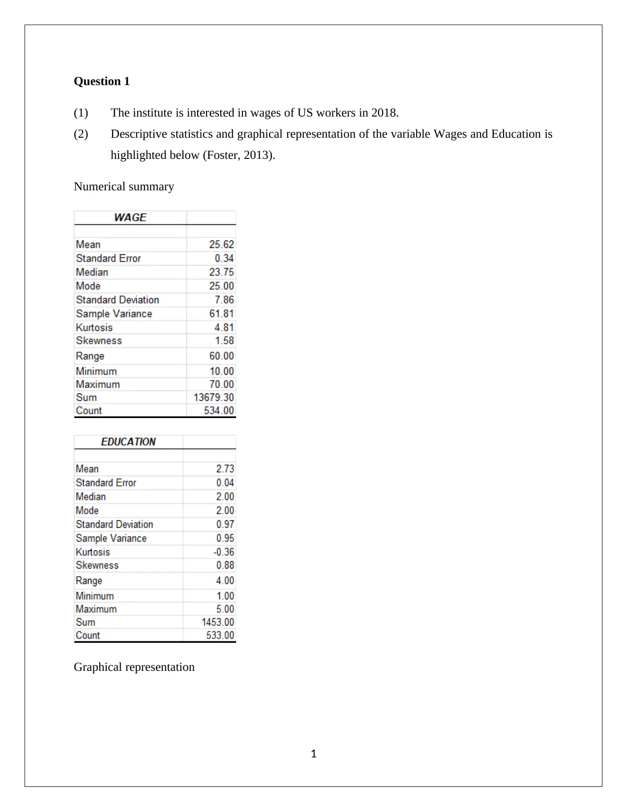
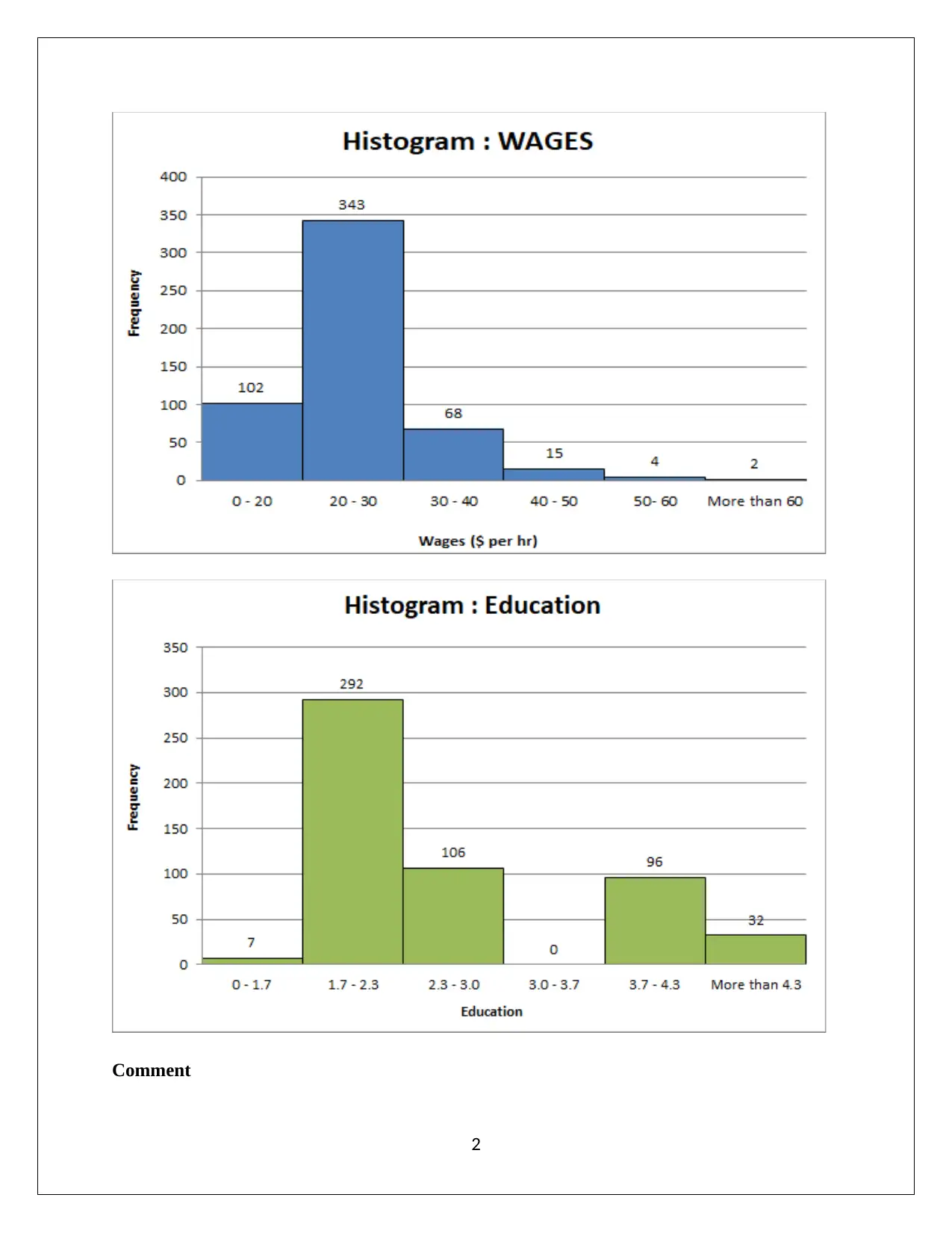
This assignment focuses on business decision-making through statistical analysis. It includes an examination of US worker wages in 2018 using descriptive statistics, graphical representations, and hypothesis testing to validate claims about wage levels and education. The analysis covers mean, median, skewness, and standard deviation of wage and education levels. Furthermore, the assignment compares prices of three-bedroom properties in New Town and Hurstville, Sydney, using hypothesis testing to determine if there's a significant difference in average house prices between the two suburbs. The conclusion provides insights for individuals making housing decisions based on budgetary constraints. Desklib offers similar solved assignments and resources for students.

PACC6008 BUSINESS DECISION MAKING
ASSIGNMENT
Student Name
[Pick the date]

Question 1
(1) The institute is interested in wages of US workers in 2018.
(2) Descriptive statistics and graphical representation of the variable Wages and Education is
highlighted below (Foster, 2013).
Numerical summary
Graphical representation
1

Comment
2

Wage Level
It is evident from the above computation that the mean hourly wage level is $25.62. Also, the
shape of the graph would be asymmetric considering that high positive skew is present which is
also validated in the histogram. This implies that there is presence of outliers on the positive side.
This can potentially distort the mean and hence central tendency may be better captured by the
median hourly wage which is $ 23.75. Also, the probability distribution related to the hourly
wage would not be normal since skew is present and also the various central tendency measures
differ in their magnitude (Rodgers, 2007). For a normal distribution, it is essential that these must
coincide. The range of the hourly wage level varies from $ 10 which is the minimum wage of
about $ 70. This is reflective of the great disparity in wages based on the underlying skill,
experience and market dynamics. Also, the standard deviation about the mean is $7.86 which
implies moderate variation in the data (Stine & Foster, 2013).
Education Level
The mean education level is 2.73 which indicates bachelor level represented by the number 3.
The median level is 2 which imply that 50% of the sample individuals have only secondary
degree. Further, skew is present in the data owing to few individuals falling in 5 bracket while
50% being restricted to secondary and primary level (Foster, 2013). The probability distribution
would not be normal owing to the asymmetric shape of the graph as highlighted in the histogram
obtained for the data provided. Besides, the deviation is data is captured from 1 to 5 where 1
highlights the lowest level i.e. primary education while 5 highlights the highest level i.e. PHD.
(3) Claim: Proportion of workers with tertiary education (Education = 3,4 &5) was 0.45.
The aim is to check the validity of the above shown claim with the help of hypothesis testing.
 Hypothesis testing for proportion would be taken into account to check the claim.
 The relevant null and alternative hypotheses are highlighted below (Rodgers, 2007):
Null hypothesis H0 : p ≤ 0.45
3

Alternative hypothesis H1 : p> 0.45
 Excel output for the hypothesis testing is shown below (Stine & Foster, 2013)
 Assuming level of significance = 5%
 Decision rule: Null hypothesis would be rejected when the p value is lower than the level of
significance.
 It this case, it can be said that p value is higher than level of significance and therefore,
insufficient evidence is present to reject the null hypothesis (Stine & Foster, 2017). Hence,
alternative hypothesis would not be accepted and final, conclusion can be made that
proportion of workers with tertiary education is lower than or equal to 0.45.
(4) Claim: Average wage per hour was $30 per hour.
The aim is to check the validity of the above shown claim with the help of hypothesis testing.
 Hypothesis testing for one sample for mean would be taken into account to check the claim.
4

 The relevant null and alternative hypotheses are highlighted below:
Null hypothesis H0 : μ=30
Alternative hypothesis H1 : μ ≠ 30
 Excel output for the hypothesis testing is shown below:
 Assuming level of significance = 5%
 Decision rule: Null hypothesis would be rejected when the p value is lower than the level of
significance (Robert, 2010).
 It this case, it can be said that p value is lower than level of significance and therefore,
sufficient evidence is present to reject the null hypothesis and to accept the alternative
hypothesis. Hence, the conclusion can be drawn that average wage rate in 2018 is different
from the 2017 wage level of $30 per hour.
Question 2
(1) Prices ($) of three bedroom property in New town and Hurstville suburb of Sydney have
been taken into consideration and is highlighted below:
5

2) The populations that we are interested in comprises of all the houses located in New Town
and Hurstville suburb which have three bedrooms. From these two populations defined above,
the sample highlighted above has been selected.
6

3) The objective of this task is to infer based on the sample prices of houses in the two suburbs if
the prices tend to differ in a significant manner or not. This would be carried out using
hypothesis testing as the enabling tool.
The requisite hypotheses are highlighted below (Stine & Foster, 2017):
Null Hypothesis: μNewTown = μHurstville i.e. the average three bedroom house prices do not differ in a
statistically significant manner from each other
Alternative Hypothesis: μNewTown ≠ μHurstville i.e. the average three bedroom house prices do differ
in a statistically significant manner from each other
The relevant test statistics would be t considering that the population standard deviation is not
known. Also, considering the alternative hypothesis, it would be correct to infer that the test
would be two tailed. Hence, a two independent sample t test needs to be performed using MS-
Excel. The relevant output is indicated below (Robert, 2010).
The two tail p value has come out as 0.00. Assuming a level of significance of 5%, it is apparent
that the p value is lower than the assumed significance level. Thus, it may be concluded that the
given evidence is sufficient to reject the null hypothesis and accept the alternative hypothesis.
4) The conclusion that can be drawn is that there is significant difference in the average price of
three bedroom houses in the two selected suburbs. Therefore, a given individual based on the
budgetary constraints can look for house in the suitable suburb.
7

References
Foster, D. (2013) Statistics for Business: Decision Making and Analysis. (2nd ed.). London:
Pearson Education Limited.
Robert, S.E. (2010) Statistics for Business: Decision Making And Analysis. Oxford: Oxford
University.
Rodgers, P. (2007) Commercial Awareness and Business Decision Making Skill: How to
understand and analyse company financial information. (4th ed.). New York:
Butterworth-Heinemann.
Stine, R. & Foster, D. (2013) Statistics for Business: Decision Making and Analysis. (2nd ed.).
London: Pearson College Division.
Stine, R. & Foster, D.P. (2017) Statistics for Business: Decision Making and Analysis. (3rd ed.).
London: Pearson.
8