Parallel Machine Scheduling: Supply Chain Cost Optimization Project

This project delves into parallel machine scheduling within the context of supply chain cost optimization. The paper introduces the problem of coordinating production and supply processes, focusing on a parallel machine scheduling model with batch delivery to two customers. The core objective is to minimize the maximum arrival time and distribution costs, utilizing a polynomial-time heuristic and worst-case analysis. The study explores the significance of cost reduction in supply chain processes, emphasizing the role of scheduling in improving profit margins and operational efficiency. It provides a background on supply chain cost problems, highlighting the relationship between supply chain management and cost constraints, and the use of techniques such as linear programming. The paper presents a parallel machine scheduling model, including definitions of key terms and notations, and illustrates the model with an example involving Gantt charts for different machine scenarios. A mathematical linear programming model is also provided, outlining symbols, descriptions, and constraints, with the goal of minimizing the maximum delivery rate (Cmax).

Parallel Machine scheduling 1
Name of School
Name of student
Professor
State
Date

Parallel Machine scheduling 2
Introduction
In the modernized produce to order supply chain processes, product manufacturers are required
to produce and supply goods and services to customers in different places. To properly
coordinate the production and the supply processes in a more detailed distribution scheduling
model, this paper focuses on the use of parallel machine scheduling model with a more definite
batch delivery system two customers from different places with the supply being done by
delivery vehicles, (Moosavirad, Kara, & Hauschild, 2014). In this scheduling model, the supply
process is made up of an order processing facility with t parallel machines serving two
customers. A set of supply chain process jobs containing s1 jobs required for customer one and
s2 jobs as are necessary for customer two are processed in the setup supply chain processing
facility with the delivery done to customers directly with no intermediate inventory required. The
main issue with the study is to determine a joint production schedule and supply activities in a
way that the activities tradeoff between the maximum arrival time required for the jobs and the
overall cost required for the distribution process is minimized (Mitra & Ranjan 2012). The
supply cost needed in the process consists of a fixed fee and a variable charge, which is
proportional to the distribution distance of the route taken to deliver the product to the customer.
To determine this, a polynomial-time heuristic with the worst-case analysis of the performance
done for the supply chain issue. If r=2 and (s-b) (s2-b) <0, the study proposes a more heuristic
with the anticipated worst-case ratio bound of 3/2. The capacity of the product supplied in any
given shipment is represented by b. overall, the worst-case rate bound in the heuristic equation
proposed in the analysis is 2-2/(m+1).
Parallel machine scheduling has been universally adopted in solving a wide range of scheduling
problems. With the current frenzy in the adoption of Just in Time manufacturing management

Parallel Machine scheduling 3
strategy, improving supply chain processes, and minimizing the overall supply chain costs is
essential to business sustainability (Metters 2018b). Therefore, scheduling supply chain activities
are becoming highly critical to reducing the total operational cost and distributing products
efficiently to the customers. Moreover, supply chain departments are directly relevant to profit
margin improvement and to increase the total income to the firm. For instance, costs involved in
moving products to the customers consume a huge chunk of the overall operations budgets
allocated in the firms. Typically, about 25% of the operations budget is consumed by supply
chain processes (Metters 2018). From this view, supply chain processes scheduling has been
considered one of the viable approaches for cutting down on the overall operations cost and
increasing income levels of the company.
In this paper, a uniform parallel machine scheduling cost problem is considered with dedicated
machines, limited budgets, and processes splitting properties, which are easily identifiable in the
supply chain management.
Background of supply chain cost problem
Over the last decade, many firms and supply chain management researchers have studied the
open relationship between the overall supply chain management and the cost constraint. Various
research approaches have been adopted to support the daily supply chain activities concerning
the product batching decisions and job sequencing issues (Pettersson, & Segerstedt, 2015). The
what-if approach has been utilized as a support system in the decision-making process
concerning the supply chain processes reengineering. Since it ensures the concerned parties can
explore the overall effects of od cost in the overall performance of supply chain management and
the impact on the whole supply chain structure (Pettersson, & Segerstedt, 2013). In the seminal
use of linear programming, it is possible to investigate and determine the overall impact of the

Parallel Machine scheduling 4
cost constraint in the supply chain activities in its efficiency and product delivery amplification
in need to increase the process rate.
In the cost constraint, activity optimization is used in solving batch sizing of the products and
sequencing the delivery activities. The impact of delivery costs on the overall performance of the
supply chain process is analyzed using the parallel machine scheduling model (Rajkumar &
Mani 2013). A continuous simulation and provide a cost optimization approach of reviewing the
total cost used to accomplish the process.
Need to measure the cost
Firms are majorly focusing on cutting costs involved in the supply chain processes with the bid
to increase the income levels. Most companies are experiencing smaller margins due to the
increased demand from the market for the provision of low-priced products. Deflationary trends
in the trading spheres globally are also exerting pressure on firms to reduce operating costs to
ensure better margins. According to Solvang (2013), one of the main issues faced by the
manufacturing firms while dealing with the supply chain process is the continuous need to
improve on the operations performances to ensure market competitiveness sustainability in the
long run.
Importance of measuring supply chain cost
With the view of cost reduction in the supply chain processes, it is essential to know the way
these associated costs are estimated. According to Quinn (2014), firms found that the best supply
chain practice is effectively moving the products to the market. These firms have a 45% supply
chain cost advantage as compare to their competitors. The delivery lead time was cut by half, and
the entire inventory days were nearly 50% as compared to those of the average competitors. And

Parallel Machine scheduling 5
the product delivery precision was found to be at 17% better than those of their customers.
Christopher and Gattorn (2015) posited the need to have a clear perspective on the supply chain
cost need. Supply chain cost savings are critical in providing firms with opportunities to increase
their profit levels.
The parallel machine scheduling model
Parallel Machine scheduling is a model used in scheduling various activities in a more elaborate
series with the same function machines with the view of optimizing the overall process. suppose
that s machines si (I = l……m) activities s operations Jj (j = l…. n) the following data can be
used in specifying all the operations for Jj
processing requirement Pg.,
the processing time of job Jj on Mi is pij,
delivery date dj,
delivery time Cj,
lateness Lj = Cj − dj,
tardiness Tj = max {0; Cj−dj},
the unit penalty Uj = 0, if Cj – dj <0; Uj=1 otherwise,
the maximum completion time, or makespan Cmax = max1 <j< n Cj,
the maximum lateness Lmax = max1 <j< nLj,
the weight wj.
Lawler et al. [10] gave a three-field classification α/β/⅄.

Parallel Machine scheduling 6
Α = describes machine environment, 2{P; Q; R}.
α =P: identical parallel machines: pij = pj for all Mi,
α =Q: uniform parallel machines: pij = pj = ri for a given speed ri of Mi,
α =R: unrelated parallel machines: pij = pj = rij for given job-dependent speeds rij of Mi.
β describes operations characteristics, 2f; pmtng.
β = pmtn: preemption is allowed, the processing of any operation may be interrupted and
resumed at a later time,
β = o: no preemption is allowed.
⅄ describes optimality criteria. In general, ⅄ {Cmax; Lmax; ∑Cj; ∑Uj; ∑Tj; ∑wjCj; ∑wjUj}.
All most all the studies were done around parallel machine scheduling under the hypothesis that
each procedure can be undertaken on in the maximum of one machine at any given time.
However, in some instances, preemptions are given room. According to the studies done by
Lawler (2012), a comprehensive analysis of parallel machine scheduling in the classification of
regular operational performances, like cost minimization, minimizing the maximum criteria,
minimizing the sum criteria of operations, and determining the precedence problem.
Example
Suppose there are seven scheduling machines and seven distribution processes to be completed
where (Pj, Sj) for all the J where 1<j<7 is provided as follows (14,5) (5,2) (12,4) (10,2) (7,3)
(15,3) (11,4). The following figure shows three Gantt charts that are related to the issue for
distribution schedules for identical or in the uniform parallel machine in which a firm operates.
In the activity Gantt chart, the number presented in the white places indicates the operation

Parallel Machine scheduling 7
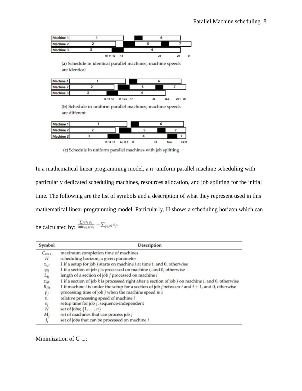
activities that require to be accomplished, and the black parts represent the setup operations. the
numbers at the bottom of the Gantt chart represent delivery time stamps, for instance. In the first
Gantt chart, machine two finishes the scheduling process at 31, while machines once and three
complete is the scheduling process in 29. Assuming that the distribution process is processed in
their index order, the distribution processes processed for the first take in each machine do not
need the setup, and there is no identifiable machine constraint. When the distribution of the
products is processed using similar machines, their scheduling span is 31, as shown in the first
Gantt chart. However, when machines with different operation speeds, for example, t2, t2, t3, are
given as 0.8, 0.9, and1 respectively, the scheduling process becomes similar, as shown in the
second Gantt chart and the overall distribution plan is 30. In this case, the distribution process
can speed up by dividing the seven distribution processes into two groups and assigning each
process group with a similar processing time of 0.73 to the third machine since the speed of the
third machine is 1. It will take 0.66 for the whole process4es in the section to be completed using
machine three and the overall distribution plan becomes 29.27. if machines 1 and 2 can be used
to meet the requirement in delivering the product to customer 7, for example., m7 = (1,2),
splitting the process will not minimize the cost and the speed of accomplishing the process.
therefore, a special consideration requires to be made on scheduling uniform parallel machines
with various effective machines used, splitting the processes and allocating enough resources is
needed.

Parallel Machine scheduling 8
In a mathematical linear programming model, a n=uniform parallel machine scheduling with
particularly dedicated scheduling machines, resources allocation, and job splitting for the initial
time. The following are the list of symbols and a description of what they represent used in this
mathematical linear programming model. Particularly, H shows a scheduling horizon which can
be calculated by:
Minimization of Cmax:

Parallel Machine scheduling 9
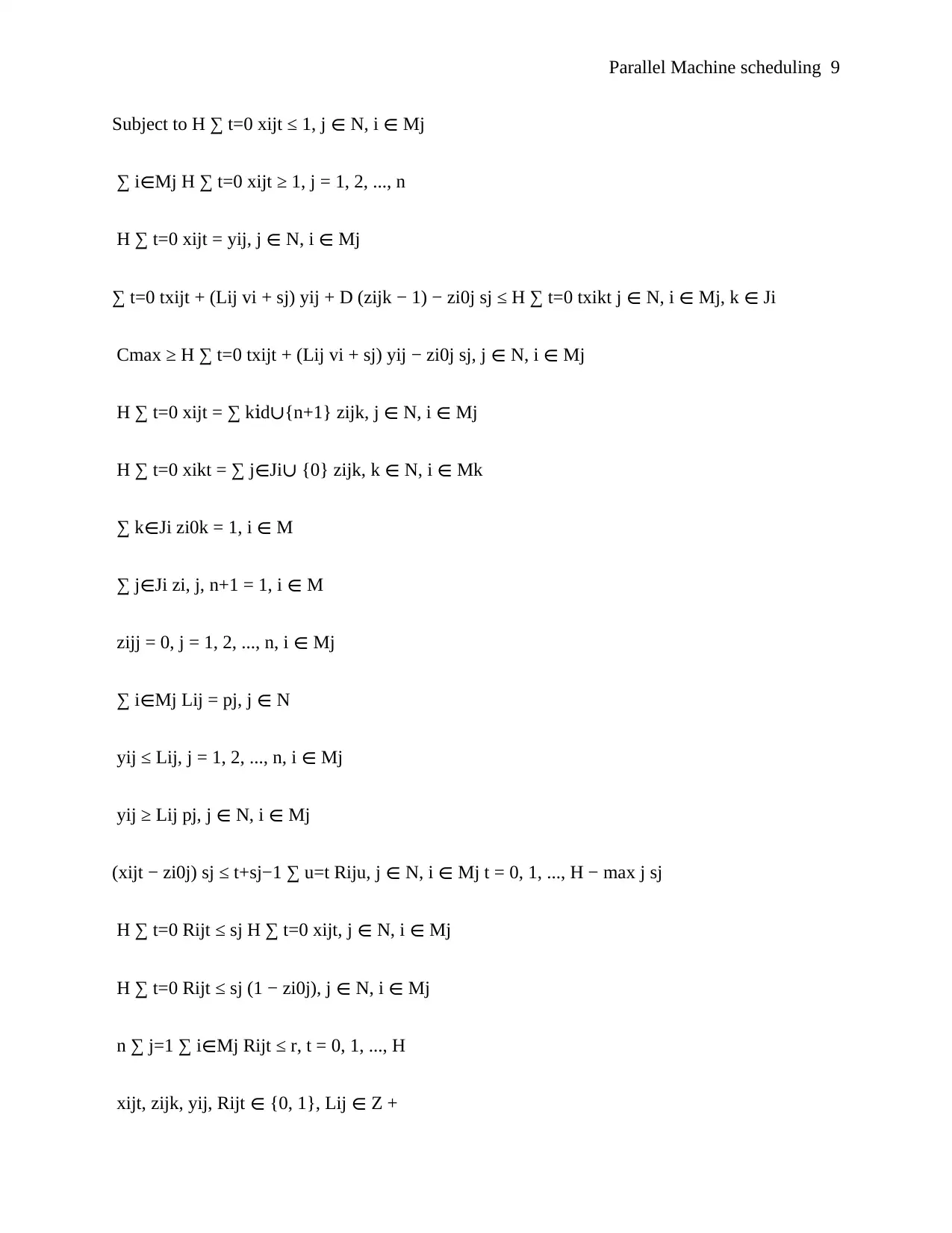
Subject to H ∑ t=0 xijt ≤ 1, j ∈ N, i ∈ Mj
∑ i∈Mj H ∑ t=0 xijt ≥ 1, j = 1, 2, ..., n
H ∑ t=0 xijt = yij, j ∈ N, i ∈ Mj
∑ t=0 txijt + (Lij vi + sj) yij + D (zijk − 1) − zi0j sj ≤ H ∑ t=0 txikt j ∈ N, i ∈ Mj, k ∈ Ji
Cmax ≥ H ∑ t=0 txijt + (Lij vi + sj) yij − zi0j sj, j ∈ N, i ∈ Mj
H ∑ t=0 xijt = ∑ kid∪{n+1} zijk, j ∈ N, i ∈ Mj
H ∑ t=0 xikt = ∑ j∈Ji∪ {0} zijk, k ∈ N, i ∈ Mk
∑ k∈Ji zi0k = 1, i ∈ M
∑ j∈Ji zi, j, n+1 = 1, i ∈ M
zijj = 0, j = 1, 2, ..., n, i ∈ Mj
∑ i∈Mj Lij = pj, j ∈ N
yij ≤ Lij, j = 1, 2, ..., n, i ∈ Mj
yij ≥ Lij pj, j ∈ N, i ∈ Mj
(xijt − zi0j) sj ≤ t+sj−1 ∑ u=t Riju, j ∈ N, i ∈ Mj t = 0, 1, ..., H − max j sj
H ∑ t=0 Rijt ≤ sj H ∑ t=0 xijt, j ∈ N, i ∈ Mj
H ∑ t=0 Rijt ≤ sj (1 − zi0j), j ∈ N, i ∈ Mj
n ∑ j=1 ∑ i∈Mj Rijt ≤ r, t = 0, 1, ..., H
xijt, zijk, yij, Rijt ∈ {0, 1}, Lij ∈ Z +

Parallel Machine scheduling 10
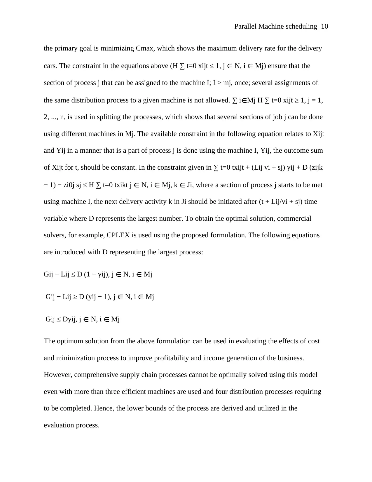
the primary goal is minimizing Cmax, which shows the maximum delivery rate for the delivery
cars. The constraint in the equations above (H ∑ t=0 xijt ≤ 1, j ∈ N, i ∈ Mj) ensure that the
section of process j that can be assigned to the machine I; I > mj, once; several assignments of
the same distribution process to a given machine is not allowed. ∑ i∈Mj H ∑ t=0 xijt ≥ 1, j = 1,
2, ..., n, is used in splitting the processes, which shows that several sections of job j can be done
using different machines in Mj. The available constraint in the following equation relates to Xijt
and Yij in a manner that is a part of process j is done using the machine I, Yij, the outcome sum
of Xijt for t, should be constant. In the constraint given in ∑ t=0 txijt + (Lij vi + sj) yij + D (zijk
− 1) − zi0j sj ≤ H ∑ t=0 txikt j ∈ N, i ∈ Mj, k ∈ Ji, where a section of process j starts to be met
using machine I, the next delivery activity k in Ji should be initiated after (t + Lij/vi + sj) time
variable where D represents the largest number. To obtain the optimal solution, commercial
solvers, for example, CPLEX is used using the proposed formulation. The following equations
are introduced with D representing the largest process:
Gij − Lij ≤ D (1 − yij), j ∈ N, i ∈ Mj
Gij − Lij ≥ D (yij − 1), j ∈ N, i ∈ Mj
Gij ≤ Dyij, j ∈ N, i ∈ Mj
The optimum solution from the above formulation can be used in evaluating the effects of cost
and minimization process to improve profitability and income generation of the business.
However, comprehensive supply chain processes cannot be optimally solved using this model
even with more than three efficient machines are used and four distribution processes requiring
to be completed. Hence, the lower bounds of the process are derived and utilized in the
evaluation process.

Parallel Machine scheduling 11
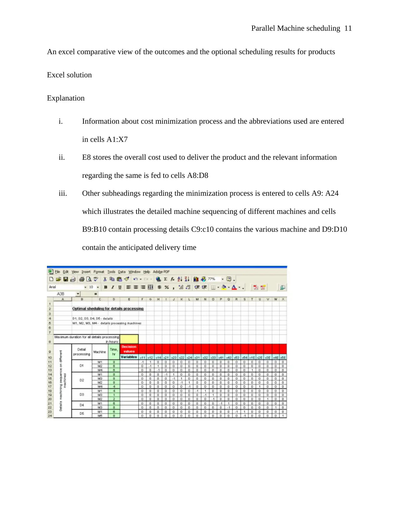
An excel comparative view of the outcomes and the optional scheduling results for products
Excel solution
Explanation
i. Information about cost minimization process and the abbreviations used are entered
in cells A1:X7
ii. E8 stores the overall cost used to deliver the product and the relevant information
regarding the same is fed to cells A8:D8
iii. Other subheadings regarding the minimization process is entered to cells A9: A24
which illustrates the detailed machine sequencing of different machines and cells
B9:B10 contain processing details C9:c10 contains the various machine and D9:D10
contain the anticipated delivery time

Parallel Machine scheduling 12
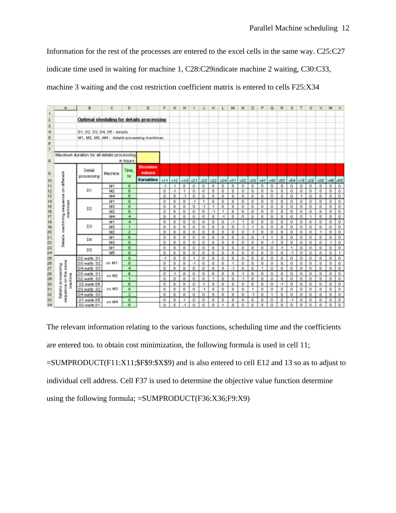
Information for the rest of the processes are entered to the excel cells in the same way. C25:C27
indicate time used in waiting for machine 1, C28:C29indicate machine 2 waiting, C30:C33,
machine 3 waiting and the cost restriction coefficient matrix is entered to cells F25:X34
The relevant information relating to the various functions, scheduling time and the coefficients
are entered too. to obtain cost minimization, the following formula is used in cell 11;
=SUMPRODUCT(F11:X11;$F$9:$X$9) and is also entered to cell E12 and 13 so as to adjust to
individual cell address. Cell F37 is used to determine the objective value function determine
using the following formula; =SUMPRODUCT(F36:X36;F9:X9)