Partial Differential Equations Assignment Solution, Analysis Module

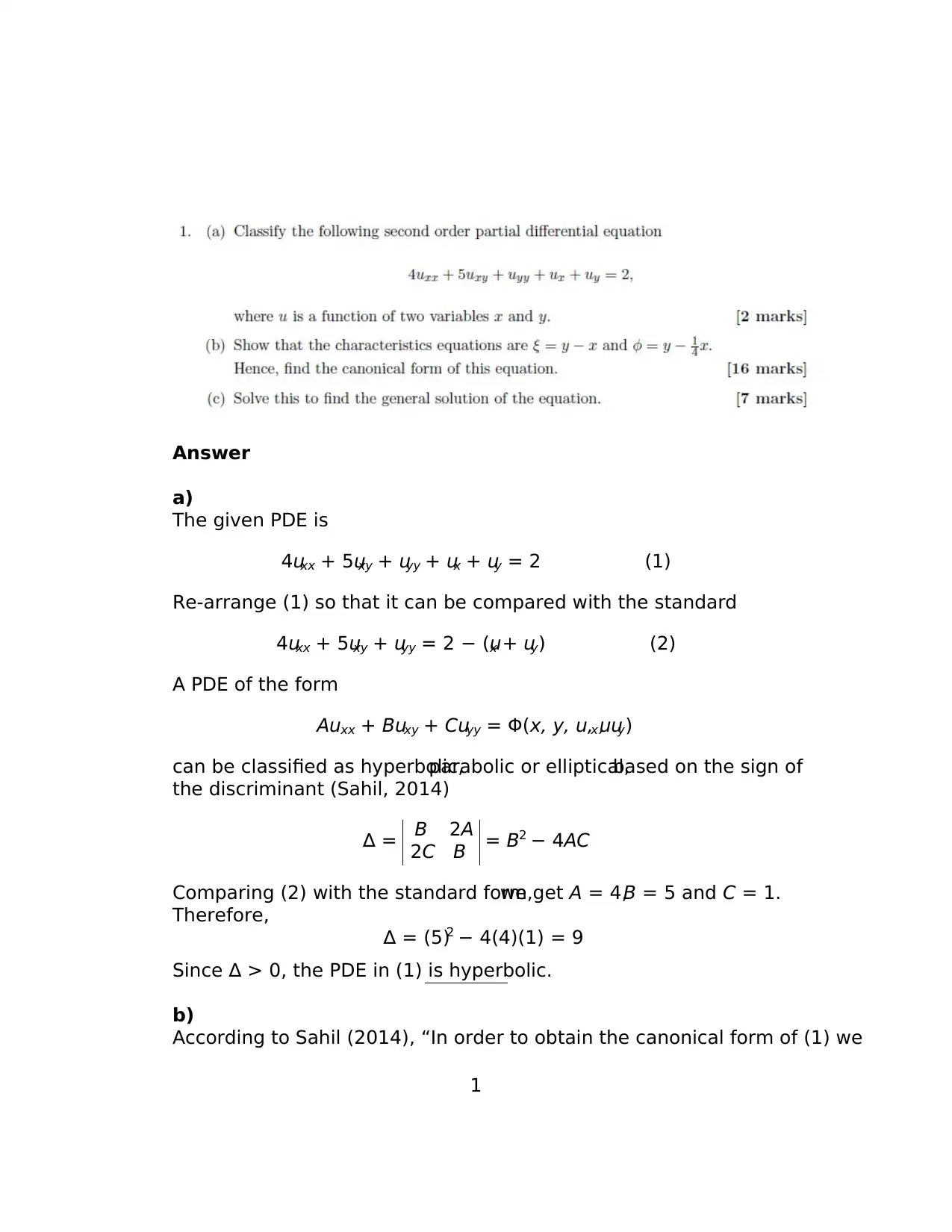
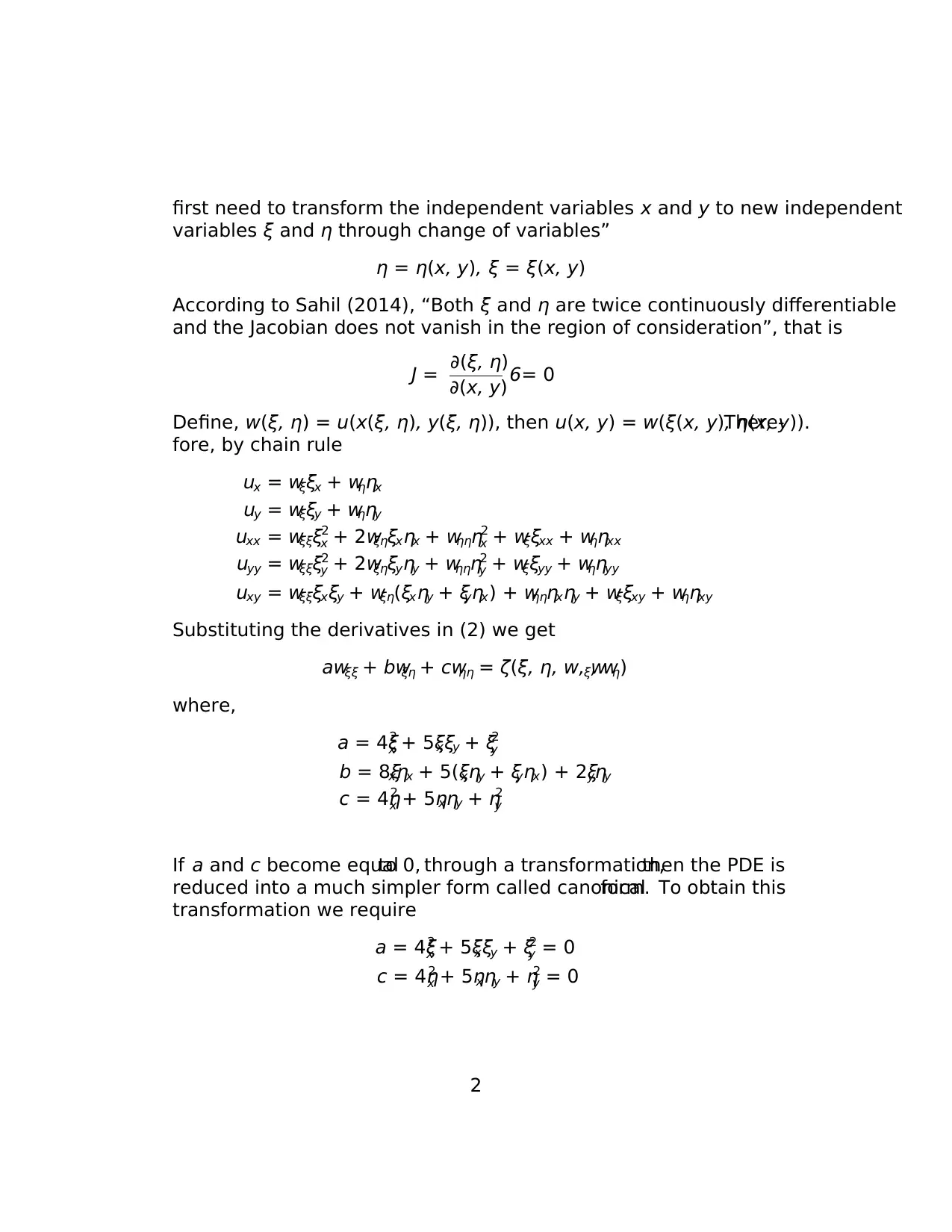
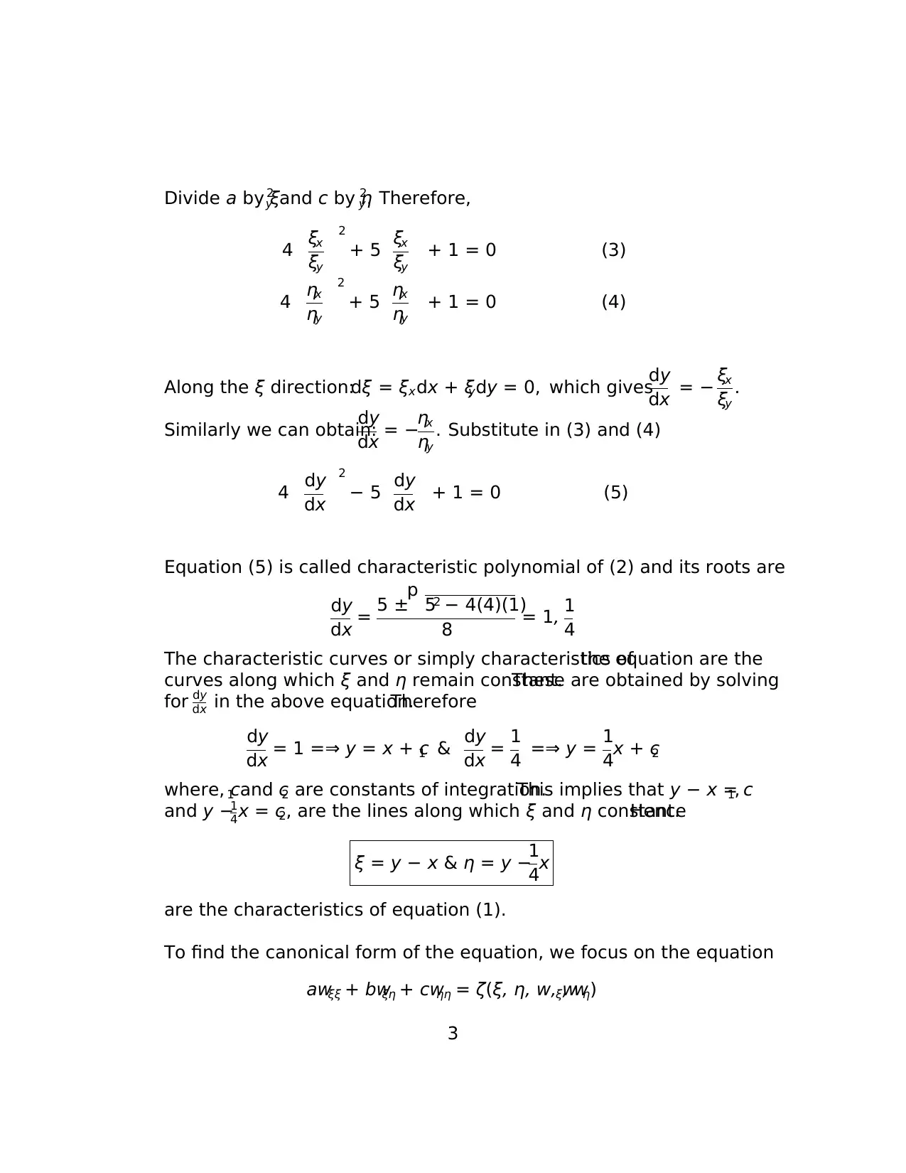
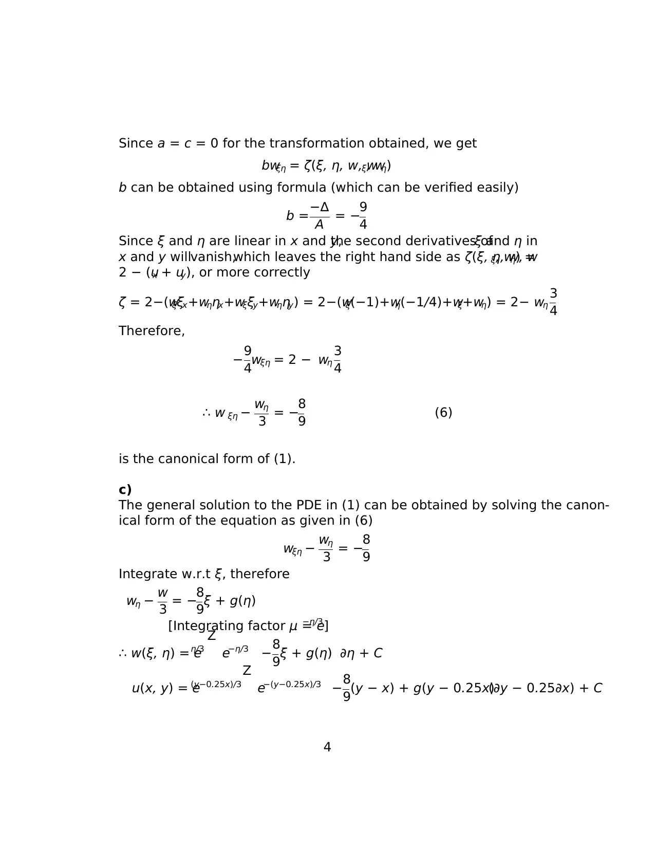
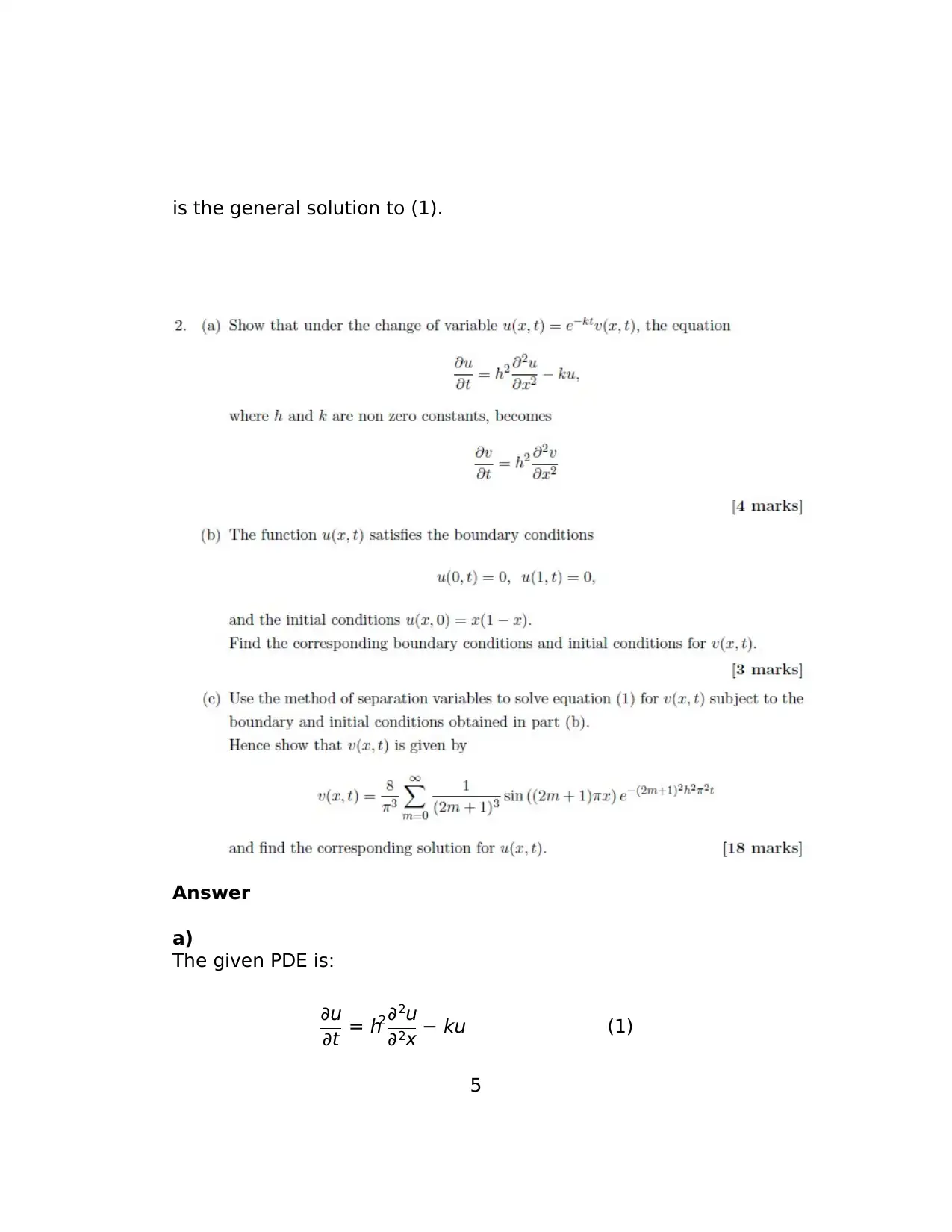
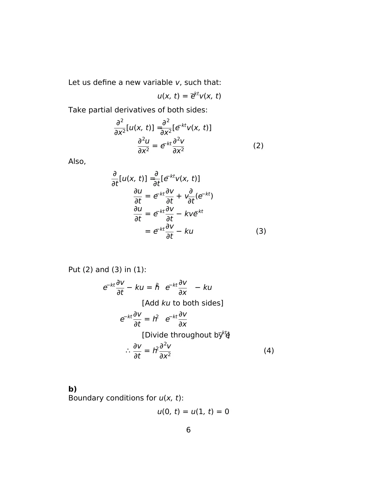
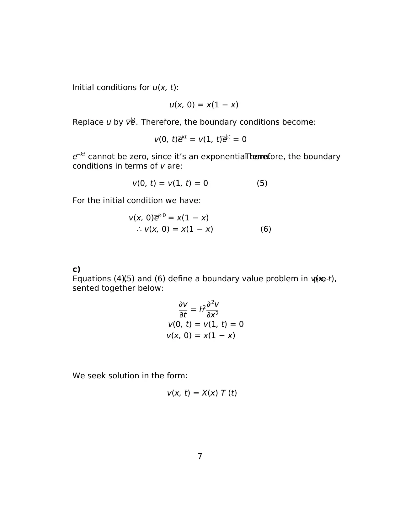
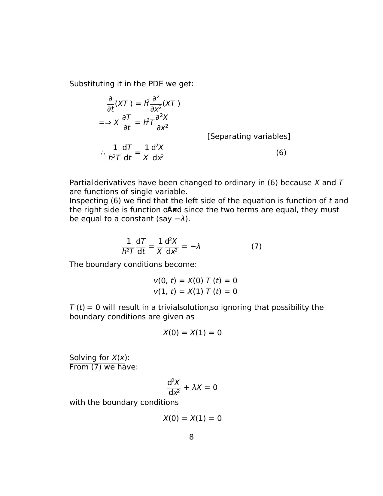
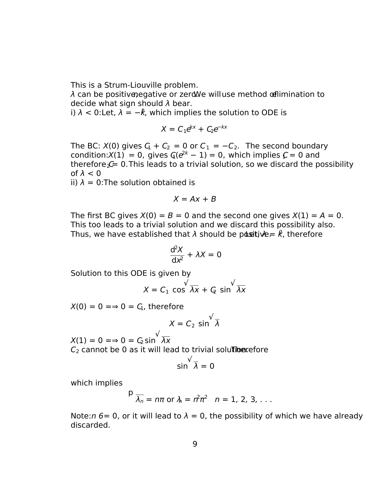
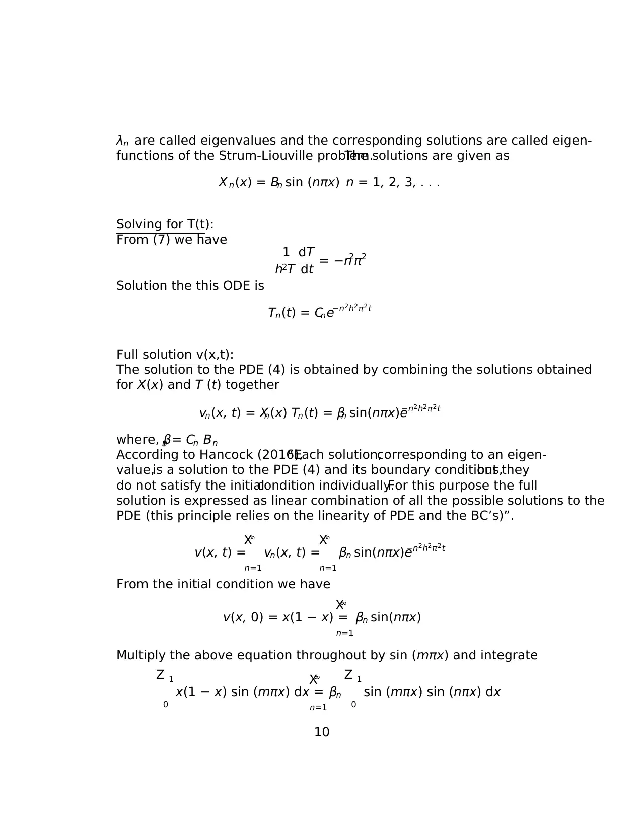
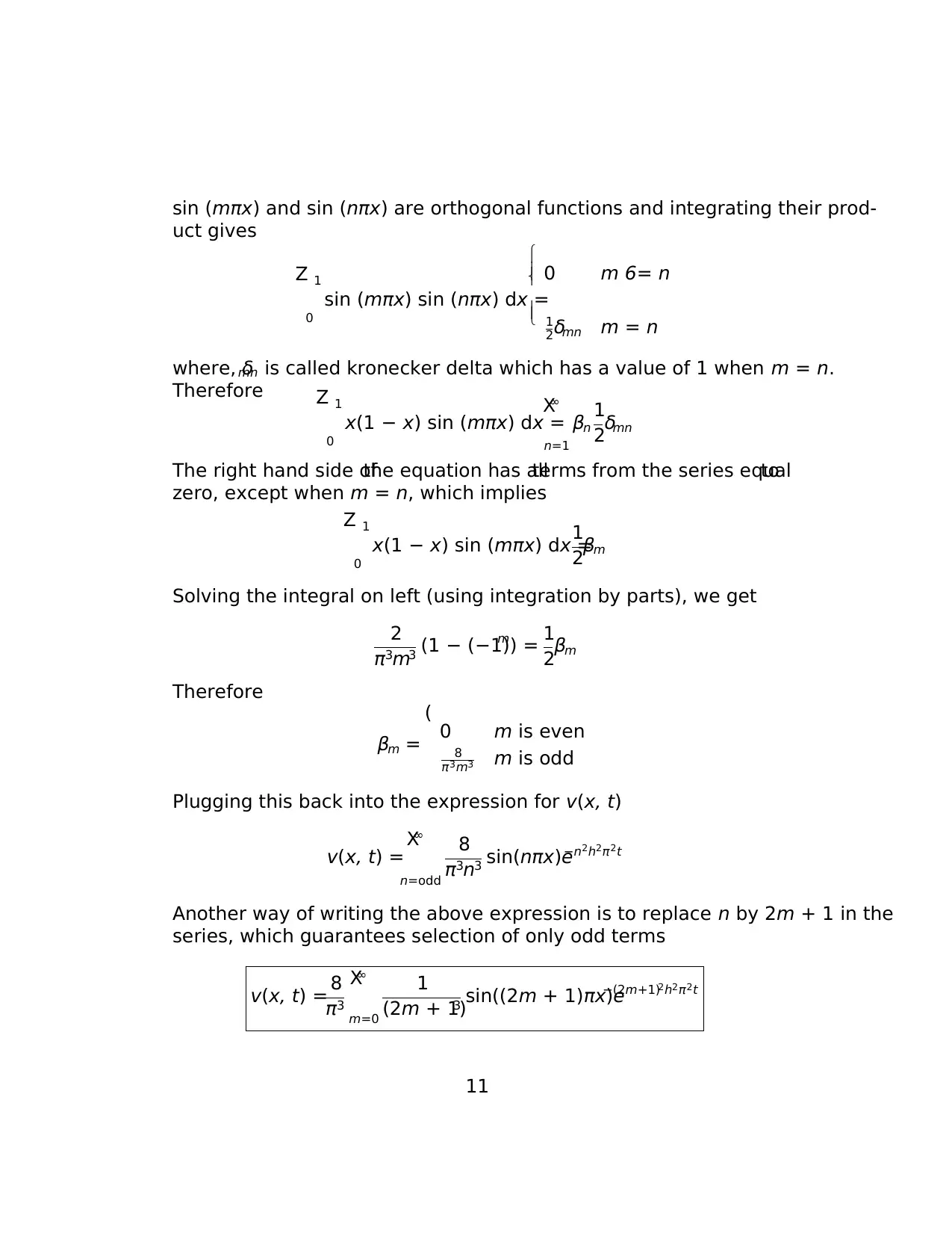
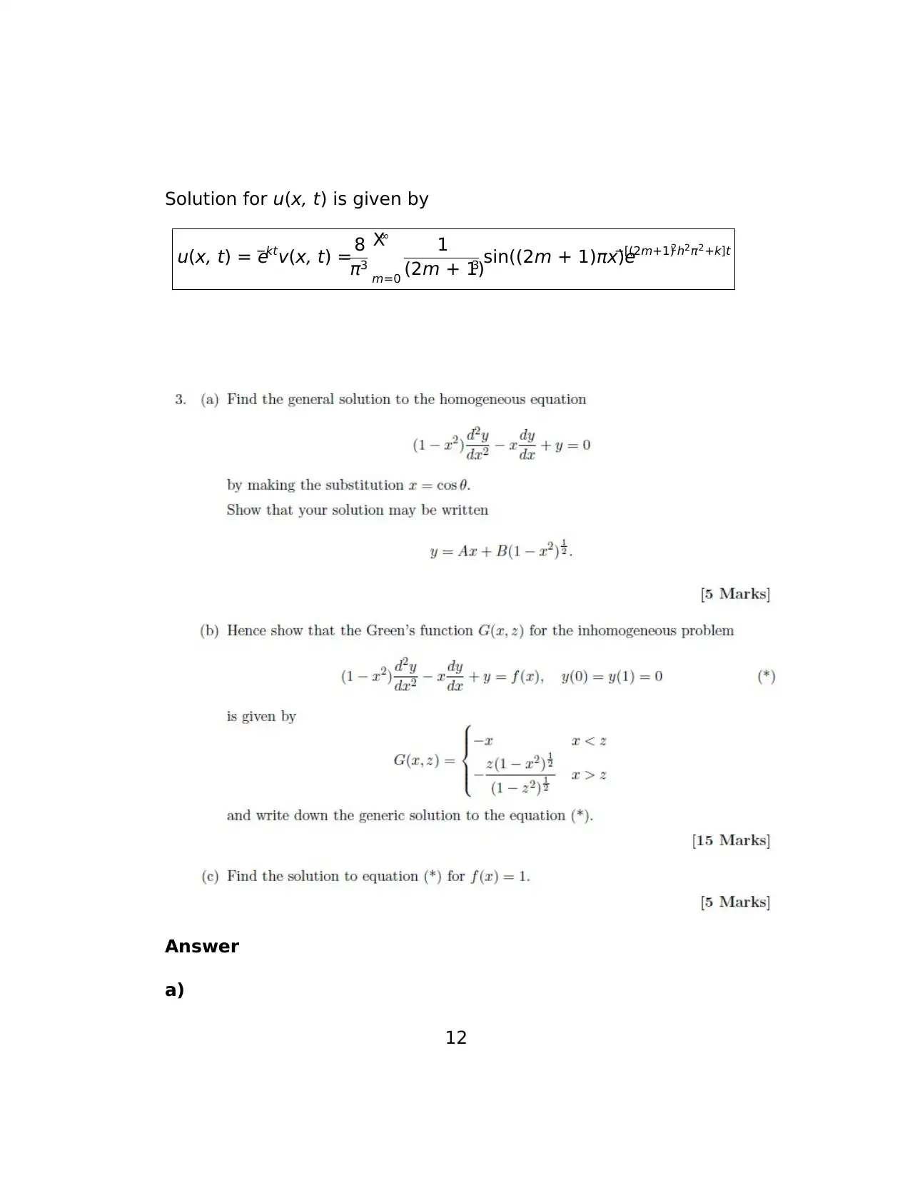
This document provides a comprehensive solution to a Partial Differential Equations (PDE) assignment. The solution addresses two main problems. The first involves classifying a given second-order PDE, determining its characteristics, finding its canonical form, and deriving the general solution. The second problem explores a heat equation with a variable transformation, deriving the boundary and initial conditions for the transformed equation. It then employs the method of separation of variables to solve the equation, including finding eigenvalues, eigenfunctions, and constructing the full solution using a linear combination of solutions to satisfy initial conditions. The assignment demonstrates a thorough understanding of PDE concepts and solution techniques.

Answer
a)
The given PDE is
4uxx + 5uxy + uyy + ux + uy = 2 (1)
Re-arrange (1) so that it can be compared with the standard
4uxx + 5uxy + uyy = 2 − (ux + uy) (2)
A PDE of the form
Auxx + Buxy + Cuyy = Φ(x, y, u, ux, uy)
can be classified as hyperbolic,parabolic or elliptical,based on the sign of
the discriminant (Sahil, 2014)
∆ = B 2A
2C B = B2 − 4AC
Comparing (2) with the standard form,we get A = 4,B = 5 and C = 1.
Therefore,
∆ = (5)2 − 4(4)(1) = 9
Since ∆ > 0, the PDE in (1) is hyperbolic.
b)
According to Sahil (2014), “In order to obtain the canonical form of (1) we
1

first need to transform the independent variables x and y to new independent
variables ξ and η through change of variables”
η = η(x, y), ξ = ξ(x, y)
According to Sahil (2014), “Both ξ and η are twice continuously differentiable
and the Jacobian does not vanish in the region of consideration”, that is
J = ∂(ξ, η)
∂(x, y)6= 0
Define, w(ξ, η) = u(x(ξ, η), y(ξ, η)), then u(x, y) = w(ξ(x, y), η(x, y)).There-
fore, by chain rule
ux = wξξx + wηηx
uy = wξξy + wηηy
uxx = wξξξ2
x + 2wξηξxηx + wηηη2
x + wξξxx + wηηxx
uyy = wξξξ2
y + 2wξηξyηy + wηηη2
y + wξξyy + wηηyy
uxy = wξξξxξy + wξη(ξxηy + ξyηx) + wηηηxηy + wξξxy + wηηxy
Substituting the derivatives in (2) we get
awξξ + bwξη + cwηη = ζ(ξ, η, w, wξ, wη)
where,
a = 4ξ2
x + 5ξxξy + ξ2
y
b = 8ξxηx + 5(ξxηy + ξyηx) + 2ξyηy
c = 4η2
x + 5ηxηy + η2
y
If a and c become equalto 0, through a transformation,then the PDE is
reduced into a much simpler form called canonicalform. To obtain this
transformation we require
a = 4ξ2
x + 5ξxξy + ξ2
y = 0
c = 4η2
x + 5ηxηy + η2
y = 0
2

Divide a by ξ2
y and c by η2
y. Therefore,
4 ξx
ξy
2
+ 5 ξx
ξy
+ 1 = 0 (3)
4 ηx
ηy
2
+ 5 ηx
ηy
+ 1 = 0 (4)
Along the ξ direction:dξ = ξxdx + ξydy = 0, which gives
dy
dx = − ξx
ξy
.
Similarly we can obtain:
dy
dx = −ηx
ηy
. Substitute in (3) and (4)
4 dy
dx
2
− 5 dy
dx + 1 = 0 (5)
Equation (5) is called characteristic polynomial of (2) and its roots are
dy
dx = 5 ±p 52 − 4(4)(1)
8 = 1, 1
4
The characteristic curves or simply characteristics ofthe equation are the
curves along which ξ and η remain constant.These are obtained by solving
for dy
dx in the above equation.Therefore
dy
dx = 1 =⇒ y = x + c1 & dy
dx = 1
4 =⇒ y = 1
4x + c2
where, c1 and c2 are constants of integration.This implies that y − x = c1,
and y −1
4x = c2, are the lines along which ξ and η constant.Hence
ξ = y − x & η = y −1
4x
are the characteristics of equation (1).
To find the canonical form of the equation, we focus on the equation
awξξ + bwξη + cwηη = ζ(ξ, η, w, wξ, wη)
3

Since a = c = 0 for the transformation obtained, we get
bwξη = ζ(ξ, η, w, wξ, wη)
b can be obtained using formula (which can be verified easily)
b =−∆
A = −9
4
Since ξ and η are linear in x and y,the second derivatives ofξ and η in
x and y willvanish,which leaves the right hand side as ζ(ξ, η, w, wξ, wη) =
2 − (ux + uy), or more correctly
ζ = 2−(wξξx+wηηx+wξξy+wηηy) = 2−(wξ(−1)+wη(−1/4)+wξ+wη) = 2− wη
3
4
Therefore,
−9
4wξη = 2 − wη
3
4
∴ w ξη − wη
3 = −8
9 (6)
is the canonical form of (1).
c)
The general solution to the PDE in (1) can be obtained by solving the canon-
ical form of the equation as given in (6)
wξη − wη
3 = −8
9
Integrate w.r.t ξ, therefore
wη − w
3 = −8
9ξ + g(η)
[Integrating factor μ = e−η/3]
∴ w(ξ, η) = eη/3
Z
e−η/3 −8
9ξ + g(η) ∂η + C
u(x, y) = e(y−0.25x)/3
Z
e−(y−0.25x)/3 −8
9(y − x) + g(y − 0.25x)(∂y − 0.25∂x) + C
4

is the general solution to (1).
Answer
a)
The given PDE is:
∂u
∂t = h2 ∂2u
∂2x − ku (1)
5

Let us define a new variable v, such that:
u(x, t) = e−ktv(x, t)
Take partial derivatives of both sides:
∂2
∂x2 [u(x, t)] =∂2
∂x2 [e−ktv(x, t)]
∂2u
∂x2 = e−kt ∂2v
∂x2 (2)
Also,
∂
∂t [u(x, t)] =∂
∂t [e−ktv(x, t)]
∂u
∂t = e−kt ∂v
∂t + v∂
∂t (e−kt)
∂u
∂t = e−kt ∂v
∂t − kve−kt
= e−kt ∂v
∂t − ku (3)
Put (2) and (3) in (1):
e−kt ∂v
∂t − ku = h2 e−kt ∂v
∂x − ku
[Add ku to both sides]
e−kt ∂v
∂t = h2 e−kt ∂v
∂x
[Divide throughout by e−kt]
∴ ∂v
∂t = h2 ∂2v
∂x2 (4)
b)
Boundary conditions for u(x, t):
u(0, t) = u(1, t) = 0
6

Initial conditions for u(x, t):
u(x, 0) = x(1 − x)
Replace u by ve−kt. Therefore, the boundary conditions become:
v(0, t)e−kt = v(1, t)e−kt = 0
e−kt cannot be zero, since it’s an exponential term.Therefore, the boundary
conditions in terms of v are:
v(0, t) = v(1, t) = 0 (5)
For the initial condition we have:
v(x, 0)e−k·0 = x(1 − x)
∴ v(x, 0) = x(1 − x) (6)
c)
Equations (4),(5) and (6) define a boundary value problem in v(x, t),pre-
sented together below:
∂v
∂t = h2 ∂2v
∂x2
v(0, t) = v(1, t) = 0
v(x, 0) = x(1 − x)
We seek solution in the form:
v(x, t) = X(x) T (t)
7

Substituting it in the PDE we get:
∂
∂t (XT ) = h2 ∂2
∂x2 (XT )
=⇒ X ∂T
∂t = h2T ∂2X
∂x2
[Separating variables]
∴ 1
h2T
dT
dt = 1
X
d2X
dx2 (6)
Partial derivatives have been changed to ordinary in (6) because X and T
are functions of single variable.
Inspecting (6) we find that the left side of the equation is function of t and
the right side is function of x.And since the two terms are equal, they must
be equal to a constant (say −λ).
1
h2T
dT
dt = 1
X
d2X
dx2 = −λ (7)
The boundary conditions become:
v(0, t) = X(0) T (t) = 0
v(1, t) = X(1) T (t) = 0
T (t) = 0 will result in a trivialsolution,so ignoring that possibility the
boundary conditions are given as
X(0) = X(1) = 0
Solving for X(x):
From (7) we have:
d2X
dx2 + λX = 0
with the boundary conditions
X(0) = X(1) = 0
8

This is a Strum-Liouville problem.
λ can be positive,negative or zero.We willuse method ofelimination to
decide what sign should λ bear.
i) λ < 0:Let, λ = −k2, which implies the solution to ODE is
X = C1ekx + C2e−kx
The BC: X(0) gives C1 + C2 = 0 or C1 = −C2. The second boundary
condition:X(1) = 0, gives C1(e2k − 1) = 0, which implies C1 = 0 and
therefore C2 = 0.This leads to a trivial solution, so we discard the possibility
of λ < 0
ii) λ = 0:The solution obtained is
X = Ax + B
The first BC gives X(0) = B = 0 and the second one gives X(1) = A = 0.
This too leads to a trivial solution and we discard this possibility also.
Thus, we have established that λ should be positive.Let, λ = k2, therefore
d2X
dx2 + λX = 0
Solution to this ODE is given by
X = C1 cos
√ λx + C2 sin√ λx
X(0) = 0 =⇒ 0 = C1, therefore
X = C2 sin√ λ
X(1) = 0 =⇒ 0 = C2 sin√ λx
C2 cannot be 0 as it will lead to trivial solution.Therefore
sin√ λ = 0
which implies
p λn = nπ or λn = n2π2 n = 1, 2, 3, . . .
Note:n 6= 0, or it will lead to λ = 0, the possibility of which we have already
discarded.
9

λn are called eigenvalues and the corresponding solutions are called eigen-
functions of the Strum-Liouville problem.The solutions are given as
X n(x) = Bn sin (nπx) n = 1, 2, 3, . . .
Solving for T(t):
From (7) we have
1
h2T
dT
dt = −n2π2
Solution the this ODE is
Tn(t) = Cne−n2h2π2t
Full solution v(x,t):
The solution to the PDE (4) is obtained by combining the solutions obtained
for X(x) and T (t) together
vn(x, t) = Xn(x) Tn(t) = βn sin(nπx)e−n2h2π2t
where, βn = Cn Bn
According to Hancock (2016),“Each solution,corresponding to an eigen-
value,is a solution to the PDE (4) and its boundary conditions,but they
do not satisfy the initialcondition individually.For this purpose the full
solution is expressed as linear combination of all the possible solutions to the
PDE (this principle relies on the linearity of PDE and the BC’s)”.
v(x, t) =
∞X
n=1
vn(x, t) =
∞X
n=1
βn sin(nπx)e−n2h2π2t
From the initial condition we have
v(x, 0) = x(1 − x) =
∞X
n=1
βn sin(nπx)
Multiply the above equation throughout by sin (mπx) and integrate
Z 1
0
x(1 − x) sin (mπx) dx =
∞X
n=1
βn
Z 1
0
sin (mπx) sin (nπx) dx
10

sin (mπx) and sin (nπx) are orthogonal functions and integrating their prod-
uct gives
Z 1
0
sin (mπx) sin (nπx) dx =



0 m 6= n
1
2δmn m = n
where, δmn is called kronecker delta which has a value of 1 when m = n.
Therefore Z 1
0
x(1 − x) sin (mπx) dx =
∞X
n=1
βn
1
2δmn
The right hand side ofthe equation has allterms from the series equalto
zero, except when m = n, which implies
Z 1
0
x(1 − x) sin (mπx) dx =
1
2βm
Solving the integral on left (using integration by parts), we get
2
π3m3 (1 − (−1)m) = 1
2βm
Therefore
βm =
(
0 m is even
8
π3m3 m is odd
Plugging this back into the expression for v(x, t)
v(x, t) =
∞X
n=odd
8
π3n3 sin(nπx)e−n2h2π2t
Another way of writing the above expression is to replace n by 2m + 1 in the
series, which guarantees selection of only odd terms
v(x, t) = 8
π3
∞X
m=0
1
(2m + 1)3 sin((2m + 1)πx)e−(2m+1)2h2π2t
11

Solution for u(x, t) is given by
u(x, t) = e−ktv(x, t) = 8
π3
∞X
m=0
1
(2m + 1)3 sin((2m + 1)πx)e−[(2m+1)2h2π2+k]t
Answer
a)
12