Report on Coherent Patient Selection in Clinical Trials Using NLP
VerifiedAdded on 2023/06/12
|30
|8160
|250
Report
AI Summary
This report discusses the application of Natural Language Processing (NLP) techniques for coherent patient selection in clinical trials, addressing the challenge of identifying patients who meet specific eligibility criteria based on their medical records. It references the 2014 i2b2/UTHealth SharedTasks and Workshop on Challenges in Natural Language Processing for Clinical Data. The report also includes a literature review of various machine learning languages and techniques applicable to this task. Key methods discussed include UMLS MetaMap for mapping biomedical text, bigrams for statistical text analysis, and tf-idf for weighting word importance in documents. The vector space model is also explored as an algebraic model for representing text documents. The goal is to streamline patient recruitment, reduce bias in clinical trials, and improve the efficiency of medical research by automating the assessment of patient eligibility.

COHERENT SELECTION FOR CLINICAL TRIALS
[Author Name(s), First M. Last, Omit Titles and Degrees]
[Institutional Affiliation(s)]
[Author Name(s), First M. Last, Omit Titles and Degrees]
[Institutional Affiliation(s)]
Paraphrase This Document
Need a fresh take? Get an instant paraphrase of this document with our AI Paraphraser
Abstract
Identifiction of patients that satify certain criteria that allows them to be plced in clincial trails
forms a fundamental aspect of medical research. This task aims to identify whether a patient
meets, does not meet, or possibly meets a selected set of eligibility criteria based on their
longitudinal records. The eligibility criteria come from real clinical trials and focus on patients’
medications, past medical histories, and whether certain events have occurred in a specified
timeframe in the patients’ records. This task uses data from the 2014 i2b2/UTHealth Shared-
Tasks and Workshop on Challenges in Natural Language Processing for Clinical Data. A
literature review on the various machine learning languages and techniques is also provided to
offer insights into these various techniques and their applicability.
Introduction
Identifiction of patients that satify certain criteria that allows them to be plced in clincial trails
forms a fundamental aspect of medical research. It is a bit of a challenge to find patients for
clincal trails owing to the sophisticated nature of the criteria of medical research which are not
easily translatable into a database query but instead require the examnation of the clcinical
narraitives that are found in the records of the patient Liu & Motoda (2012). This tends to take a
lot of timeespecially for medical resrecher who are intending to recurit patients and thus
researchers are usually linited to patients who are directed towards a cetain trial or seek for trial
on their own. Recruitment from particular places or by particular people can result in selection
bias towards certain populations which in turn can bias the results of the study Robert (2014).
Developing NLP systems that can automatically assess if a patient is eligible for a study can both
reduce the time it takes to recruit patients, and help remove bias from clinical trials.
Identifiction of patients that satify certain criteria that allows them to be plced in clincial trails
forms a fundamental aspect of medical research. This task aims to identify whether a patient
meets, does not meet, or possibly meets a selected set of eligibility criteria based on their
longitudinal records. The eligibility criteria come from real clinical trials and focus on patients’
medications, past medical histories, and whether certain events have occurred in a specified
timeframe in the patients’ records. This task uses data from the 2014 i2b2/UTHealth Shared-
Tasks and Workshop on Challenges in Natural Language Processing for Clinical Data. A
literature review on the various machine learning languages and techniques is also provided to
offer insights into these various techniques and their applicability.
Introduction
Identifiction of patients that satify certain criteria that allows them to be plced in clincial trails
forms a fundamental aspect of medical research. It is a bit of a challenge to find patients for
clincal trails owing to the sophisticated nature of the criteria of medical research which are not
easily translatable into a database query but instead require the examnation of the clcinical
narraitives that are found in the records of the patient Liu & Motoda (2012). This tends to take a
lot of timeespecially for medical resrecher who are intending to recurit patients and thus
researchers are usually linited to patients who are directed towards a cetain trial or seek for trial
on their own. Recruitment from particular places or by particular people can result in selection
bias towards certain populations which in turn can bias the results of the study Robert (2014).
Developing NLP systems that can automatically assess if a patient is eligible for a study can both
reduce the time it takes to recruit patients, and help remove bias from clinical trials.
However, matching patients to selection criteria is not a trivial task for machines, due to the
complexity the criteria often exhibit. This shared task aims to identify whether a patient meets,
does not meet, or possibly meets a selected set of eligibility criteria based on their longitudinal
records. The eligibility criteria come from real clinical trials and focus on patients’ medications,
past medical histories, and whether certain events have occurred in a specified timeframe in the
patients’ records Alpaydin (2014). This task uses data from the 2014 i2b2/UTHealth Shared-
Tasks and Workshop on Challenges in Natural Language Processing for Clinical Data, with tasks
on de-identification and heart disease risk factors. The data is composed of nearly 202 sets of
longitudinal patient records, annotated by medical professionals to determine if each patient
matches a list of 13 selection criteria. These criteria include determining whether the patient has
taken a dietary supplement (excluding Vitamin D) in the past 2 months, whether the patient has a
major diabetes-related complication, and whether the patient has advanced cardiovascular
disease.
All the files have been annotated at the document level to indicate whether the patient meets or
do not meet each criterion. The gold standard annotations will provide the category of each
patient for each criterion Alpaydin (2014). Participants will be evaluated on the predicted
category of each patient in the held-out test data. The data for this task is provided by Partners
HealthCare. All records have been fully de-identified and manually annotated for whether they
meet, possibly meet, or do not meet clinical trial eligibility criteria. The evaluation for both NLP
tasks will be conducted using withheld test data in which the participating teams are asked to
stop development as soon as they download the test data. Each team is allowed to upload
(through this website) up to three system runs for each of these tracks. System output is to be
⊘ This is a preview!⊘
Do you want full access?
Subscribe today to unlock all pages.
Trusted by 1+ million students worldwide
submitted in the exact format of the ground truth annotations, which will be provided by the
organizers Paik (2013, July).
Participants are asked to submit a 500-word long abstract describing their methodologies.
Abstracts may also have a graphical summary of the proposed architecture. The authors of either
top performing systems or particularly novel approaches will be invited to present or
demonstrate their systems at the workshop Liu & Motoda (2012). A special issue of a journal
will be organized following the workshop.
UMLS MetaMap
This is a program that is highly configurable and was developed for the purposes of mapping
biomedical text to UMLS Metathesaurus or in equal measure makes discoveries on the concept
of Metathesaurus that is referred to in a text. UMLS MetaMap makes used of an approach of
knowledge-intensive that is pegged on symbolic natural language processing as well as
computational linguistic techniques Alpaydin (2014). Other than finding its applications in IR
and data mining applications, MetaMap is acknowledged as one of the foundations of Medical
Text Indexer (MTI) of the National Library Medicine. The Medical Text Indexer is applied both
in semiautomatic as well as entirely automatic indexing of the literature of biomedicine at the
National Library Medicine.
An improved version of MetaMap is available called MetaMap2016 V2 that has come with
numerous new features having special purposes that are aimed at improving the performance of
specific input types. There are also provided JSON output besides the XML output. Among the
benefits that come with MetaMap2016 V2 include:
Paraphrase This Document
Need a fresh take? Get an instant paraphrase of this document with our AI Paraphraser
Suppression of Numerical concepts: There are some numerical concepts of certain
Sematic Type that have been found to inject limited value to an entity of a biomedical
name recognition application. Through MetaMap2016 V2 such unnecessary and
irrelevant concepts are automatically suppressed Goeuriot et al (2014, September).
JSON Output generation: MetaMap2016 V2 is able to produce an output of JSON
Processing of data in tables: Through MetaMap2016 V2 is possible to identify concepts
of UMLS in a better and more efficient way as they are found in tabular data.
Improved Conjunction Handling: There is provision for an improvement in the handling
of conjunction by MetaMap2016 V2.
Bigram
Also called a diagram, a bigram is a sequence made up of two elements that are adjacent to each
other from a string of tokens which are basically letter, words or syllables. It is an n-gram for
n=2. The distribution frequency of each of the bigram in the string is applied in simple statistical
analysis of texts in various applications among them speech recognition, computational
linguistics and cystography among others. Guppy bigrams or simply skipping bigrams are pairs
of words that enable gaps (may be by avoiding the use of connecting words or through
permitting some dependencies of simulation as is the case with a dependency grammar)
Rocktäschel, Weidlich & Leser (2012).
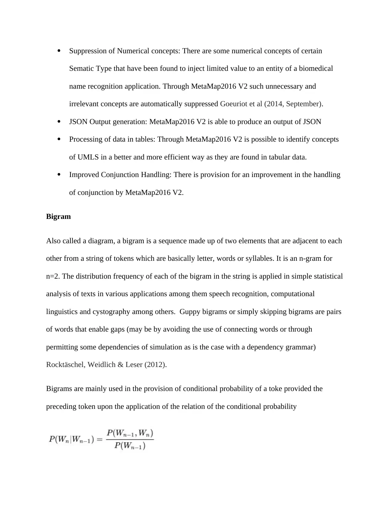
Bigrams are mainly used in the provision of conditional probability of a toke provided the
preceding token upon the application of the relation of the conditional probability
Sematic Type that have been found to inject limited value to an entity of a biomedical
name recognition application. Through MetaMap2016 V2 such unnecessary and
irrelevant concepts are automatically suppressed Goeuriot et al (2014, September).
JSON Output generation: MetaMap2016 V2 is able to produce an output of JSON
Processing of data in tables: Through MetaMap2016 V2 is possible to identify concepts
of UMLS in a better and more efficient way as they are found in tabular data.
Improved Conjunction Handling: There is provision for an improvement in the handling
of conjunction by MetaMap2016 V2.
Bigram
Also called a diagram, a bigram is a sequence made up of two elements that are adjacent to each
other from a string of tokens which are basically letter, words or syllables. It is an n-gram for
n=2. The distribution frequency of each of the bigram in the string is applied in simple statistical
analysis of texts in various applications among them speech recognition, computational
linguistics and cystography among others. Guppy bigrams or simply skipping bigrams are pairs
of words that enable gaps (may be by avoiding the use of connecting words or through
permitting some dependencies of simulation as is the case with a dependency grammar)
Rocktäschel, Weidlich & Leser (2012).
Bigrams are mainly used in the provision of conditional probability of a toke provided the
preceding token upon the application of the relation of the conditional probability
Applications
They are applied in what is termed as one of the most successful models of language in
the recognition of speech in which they act as a special case of n-gram.
The attacks of bigram frequency are usable in cryptography for solving cryptograms Del,
López, Benítez, & Herrera (2014)
One of the approaches in statistical language identification
Bigrams are involved in some of the activities of recreational linguistics or logo logy
tf-idf
When used in information retrieval, tf-idf or TFIDF is an abbreviation for term frequency-
inverse document frequency and refers to a numerical statistics that is meant for reflecting the
importance of a word in any document that is available in a collection or a corpus. It is normally
adopted as weighting factors in searches involving the retrieval of information, user modeling as
well as text mining Alpaydin (2014). There is proportional increase in the value of tf-idf with the
frequency of appearance of a word in a document and is usually offset by the now frequent the
word is in the corpus. This assists in the adjustment owing to the fact that some words generally
appear more frequently.
The aim of using tf-idf as opposed to raw frequencies of occurrence of any token in a provided
document is scaling down the effects of the tokens that may be occur more frequently in a
specific corpus and which are thus less informative in empirical terms that the features that take
place in a small fraction of the training corpus Alpaydin (2014).
Computation of tf-idf is done using the formula t is tf-idf (d, t)=tf (t)*idf (d,t) while the idf is
computed rom the from idf(d,t)=log (n/df(d,t))+1 and this is applicable under the conditions (if
⊘ This is a preview!⊘
Do you want full access?
Subscribe today to unlock all pages.
Trusted by 1+ million students worldwide
smooth_idf=False) in which n is the total amount of the documents and df(d,t) as the frequency
of the document; the frequency of the document refers to the number of documents of d that have
the term t. the addition of 1 in the idf of the equation shown is that in case of terms with zero idf
which is the terms that are found in all the documents in a single training set, not be all ignored
Witten et al (2016). It should be noted that there is a difference between the formula of idf listed
in this paper and that found in standard textbook notations which in most cases define idf as
idf(d, t)=log (n/(df(d, t+1))) the condition here remains if smooth_idf=True which is the default
conditions, there is addition of 1 to both the numerator and the denominator of the idf in a
manner suggesting that there was access to an extra document every time there was a collection
just once thereby preventing zero divisions: idf (d,t)=log (1+n)/(1+df (d,t))+1 Paik (2013, July)
These formulas that are furthermore used in the computation of the tf and idf are a factor of the
settings of the parameter which are in correspondence with the SMART notation that is deployed
in IR as follows:
Tf is by default n (natural), l which is the logarithmic when sublinear_tf=True. Idf is found to be
t when use_idf is provided, n (none) otherwise. The normalization is found to be c (cosine) at
norm= ‘12’, n (none) when norm=none Paik (2013, July).
There is a significant difference between sentiment analysis and tf-idf even though all of them
are treated as techniques for classification for text, they have distinct goals. While sentiment
analysis is aiming at classification of documents based on opinions such as negative and positive,
tf-idf classifies documents into various categories that are within the very documents.
Paraphrase This Document
Need a fresh take? Get an instant paraphrase of this document with our AI Paraphraser
Applications of tf-idf
This algorithm tends to be more useful in cases where there is large set of document that is
supposed to be characterized. It is simple as one does not need to train a model before time but
instead it will just automatically account for the variations in the lengths of the document
Rocktäschel et al (2012).
Vector Space Model Representation
Also called term vector model, vector space model is an algebraic model that is used in the
representation of text documents or any objects generally as vectors of identifiers for example in
terms of index. Vector space model is applied in filtering of information, indexing, and retrieval
and relevancy rankings Alpaydin (2014). The model was first applied in the SMART
Information Retrieval System.
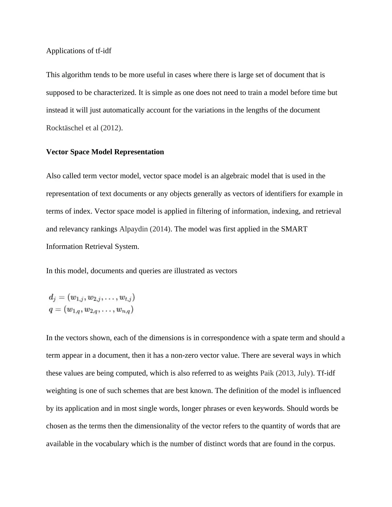
In this model, documents and queries are illustrated as vectors
In the vectors shown, each of the dimensions is in correspondence with a spate term and should a
term appear in a document, then it has a non-zero vector value. There are several ways in which
these values are being computed, which is also referred to as weights Paik (2013, July). Tf-idf
weighting is one of such schemes that are best known. The definition of the model is influenced
by its application and in most single words, longer phrases or even keywords. Should words be
chosen as the terms then the dimensionality of the vector refers to the quantity of words that are
available in the vocabulary which is the number of distinct words that are found in the corpus.
This algorithm tends to be more useful in cases where there is large set of document that is
supposed to be characterized. It is simple as one does not need to train a model before time but
instead it will just automatically account for the variations in the lengths of the document
Rocktäschel et al (2012).
Vector Space Model Representation
Also called term vector model, vector space model is an algebraic model that is used in the
representation of text documents or any objects generally as vectors of identifiers for example in
terms of index. Vector space model is applied in filtering of information, indexing, and retrieval
and relevancy rankings Alpaydin (2014). The model was first applied in the SMART
Information Retrieval System.
In this model, documents and queries are illustrated as vectors
In the vectors shown, each of the dimensions is in correspondence with a spate term and should a
term appear in a document, then it has a non-zero vector value. There are several ways in which
these values are being computed, which is also referred to as weights Paik (2013, July). Tf-idf
weighting is one of such schemes that are best known. The definition of the model is influenced
by its application and in most single words, longer phrases or even keywords. Should words be
chosen as the terms then the dimensionality of the vector refers to the quantity of words that are
available in the vocabulary which is the number of distinct words that are found in the corpus.
Applications
By the use of the assumption of similarity of documents theory, it os possible to compute the
relevance rankings of documents available in a keyword search. This is achieved through making
a comparison between the angles of deviation between each of the documents vector and the
vector of the original query in which the query is represented as the very vector kind as the
documents Alpaydin (2014).
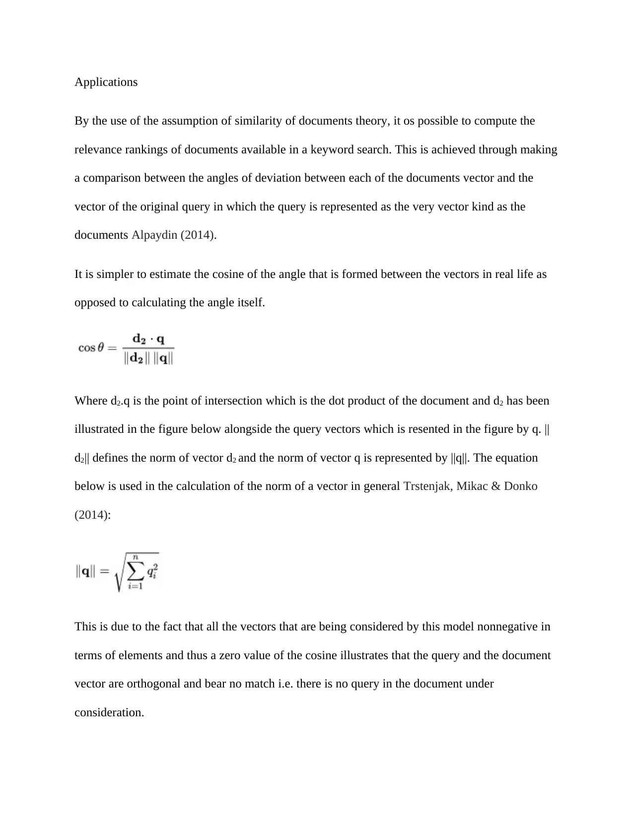
It is simpler to estimate the cosine of the angle that is formed between the vectors in real life as
opposed to calculating the angle itself.
Where d2.q is the point of intersection which is the dot product of the document and d2 has been
illustrated in the figure below alongside the query vectors which is resented in the figure by q. ||
d2|| defines the norm of vector d2 and the norm of vector q is represented by ||q||. The equation
below is used in the calculation of the norm of a vector in general Trstenjak, Mikac & Donko
(2014):
This is due to the fact that all the vectors that are being considered by this model nonnegative in
terms of elements and thus a zero value of the cosine illustrates that the query and the document
vector are orthogonal and bear no match i.e. there is no query in the document under
consideration.
By the use of the assumption of similarity of documents theory, it os possible to compute the
relevance rankings of documents available in a keyword search. This is achieved through making
a comparison between the angles of deviation between each of the documents vector and the
vector of the original query in which the query is represented as the very vector kind as the
documents Alpaydin (2014).
It is simpler to estimate the cosine of the angle that is formed between the vectors in real life as
opposed to calculating the angle itself.
Where d2.q is the point of intersection which is the dot product of the document and d2 has been
illustrated in the figure below alongside the query vectors which is resented in the figure by q. ||
d2|| defines the norm of vector d2 and the norm of vector q is represented by ||q||. The equation
below is used in the calculation of the norm of a vector in general Trstenjak, Mikac & Donko
(2014):
This is due to the fact that all the vectors that are being considered by this model nonnegative in
terms of elements and thus a zero value of the cosine illustrates that the query and the document
vector are orthogonal and bear no match i.e. there is no query in the document under
consideration.
⊘ This is a preview!⊘
Do you want full access?
Subscribe today to unlock all pages.
Trusted by 1+ million students worldwide
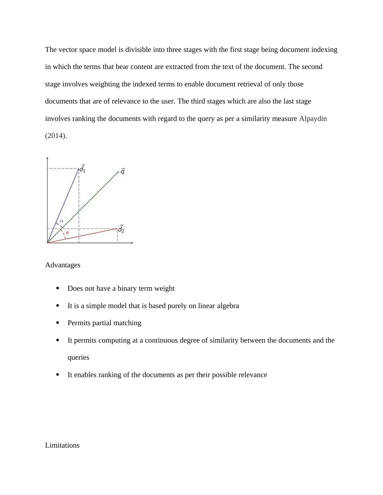
The vector space model is divisible into three stages with the first stage being document indexing
in which the terms that bear content are extracted from the text of the document. The second
stage involves weighting the indexed terms to enable document retrieval of only those
documents that are of relevance to the user. The third stages which are also the last stage
involves ranking the documents with regard to the query as per a similarity measure Alpaydin
(2014).
Advantages
Does not have a binary term weight
It is a simple model that is based purely on linear algebra
Permits partial matching
It permits computing at a continuous degree of similarity between the documents and the
queries
It enables ranking of the documents as per their possible relevance
Limitations
Paraphrase This Document
Need a fresh take? Get an instant paraphrase of this document with our AI Paraphraser
It has an intuitive weighting which is not very formal
It is poor in the representation of long documents due to their poor similarity values
There is loss of order of appearance in the vector space representation as was in the
document Chandrashekar & Sahin (2014)
It has a theoretical assumption that terms are independent statistically
It has sematic sensitivity i.e. documents that have similar context but distinct term
vocabulary cannot be associated and thus bringing about a false negative match.
Feature Selection
Feature Selection forms an integral step in data processing that is done just the application of a
learning algorithm. The complexity of the computation is the main issue that is taken into
consideration when a proposal is being made on a method of feature selection. In most case, a
fast feature selection process is unable to search rough the space of the feature subset thus the
accuracy of the classification is found to be reduced Alpaydin (2014). Also known as variable
selection, variable subset selection and attribute selection, feature selection n defines the process
through which a subset of the appropriate and relevant features is selected to be used in the
model construction.
The main role of feature selection is the elimination of the irrelevant and redundant features.
Irrelevant features are features that are treated to be providing information that is of no use with
regard to the data while redundant features are those that are no longer providing information
apart from the currently chosen features. In other terms, redundant features offer information
which is of importance to the data set even though the same information is already provided by
the currently chosen features Chandrashekar & Sahin (2014).
An example of such is the year of birth as well as the age which provide the very information
about a person. Redundant and irrelevant feature have the potential of lowering the accuracy of
learning and the model quality achieved by the learning algorithm. There are numerous
proposals that have been made in an attempt to more accurately and efficiently apply the learning
algorithms Alpaydin (2014). Such proposals reduce the dimensionality for example relief, CFS,
FOCUS. Through the removal of the irrelevant information and minimizing noise levels, the
accuracy and efficiency of leaning algorithms can significantly be improved. Feature selection
has attracted special interests especially in areas of research that call for high dimensional
datasets such as text processing, combinational chemistry and gene expression.
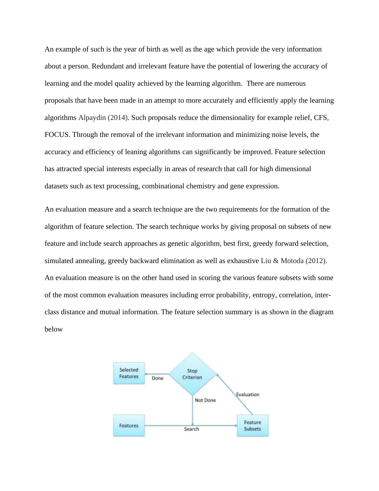
An evaluation measure and a search technique are the two requirements for the formation of the
algorithm of feature selection. The search technique works by giving proposal on subsets of new
feature and include search approaches as genetic algorithm, best first, greedy forward selection,
simulated annealing, greedy backward elimination as well as exhaustive Liu & Motoda (2012).
An evaluation measure is on the other hand used in scoring the various feature subsets with some
of the most common evaluation measures including error probability, entropy, correlation, inter-
class distance and mutual information. The feature selection summary is as shown in the diagram
below
about a person. Redundant and irrelevant feature have the potential of lowering the accuracy of
learning and the model quality achieved by the learning algorithm. There are numerous
proposals that have been made in an attempt to more accurately and efficiently apply the learning
algorithms Alpaydin (2014). Such proposals reduce the dimensionality for example relief, CFS,
FOCUS. Through the removal of the irrelevant information and minimizing noise levels, the
accuracy and efficiency of leaning algorithms can significantly be improved. Feature selection
has attracted special interests especially in areas of research that call for high dimensional
datasets such as text processing, combinational chemistry and gene expression.
An evaluation measure and a search technique are the two requirements for the formation of the
algorithm of feature selection. The search technique works by giving proposal on subsets of new
feature and include search approaches as genetic algorithm, best first, greedy forward selection,
simulated annealing, greedy backward elimination as well as exhaustive Liu & Motoda (2012).
An evaluation measure is on the other hand used in scoring the various feature subsets with some
of the most common evaluation measures including error probability, entropy, correlation, inter-
class distance and mutual information. The feature selection summary is as shown in the diagram
below
⊘ This is a preview!⊘
Do you want full access?
Subscribe today to unlock all pages.
Trusted by 1+ million students worldwide
1 out of 30

Your All-in-One AI-Powered Toolkit for Academic Success.
+13062052269
info@desklib.com
Available 24*7 on WhatsApp / Email
![[object Object]](/_next/static/media/star-bottom.7253800d.svg)
Unlock your academic potential
Copyright © 2020–2026 A2Z Services. All Rights Reserved. Developed and managed by ZUCOL.