Microeconomics Assignment: Perfect Competition to Oligopoly Analysis

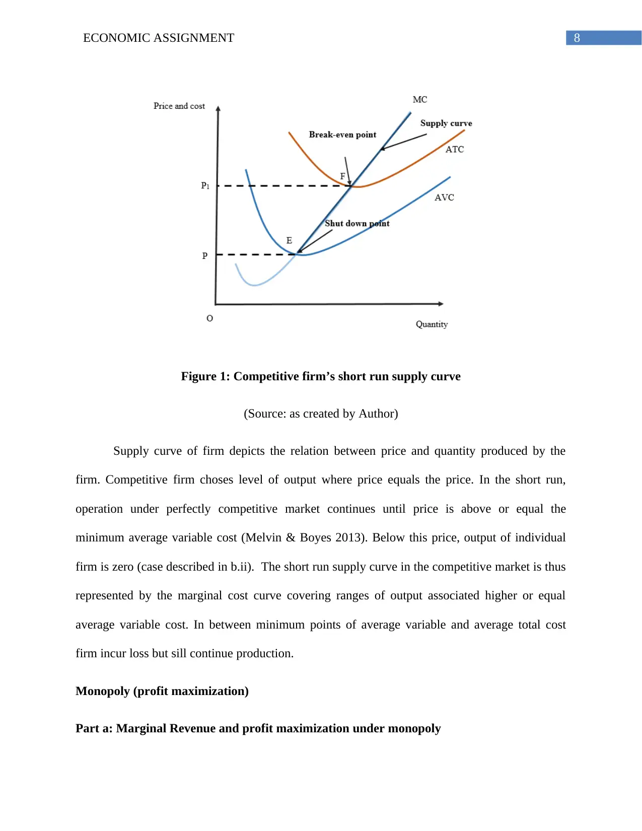
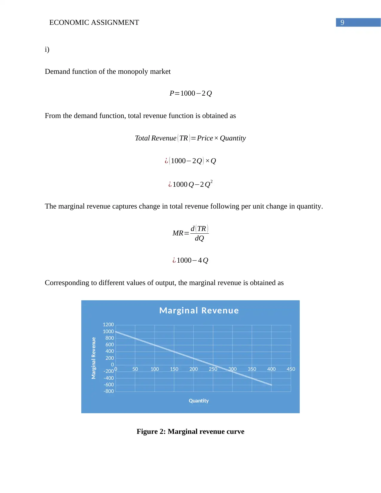
This economics assignment provides a comprehensive analysis of various market structures, including perfect competition, monopoly, monopolistic competition, and oligopoly. The assignment begins with an examination of perfect competition, exploring its assumptions, profit maximization, and short-run and long-run equilibrium. It then delves into the concept of shutdown points and the construction of short-run supply curves. The analysis proceeds to explore monopoly markets, covering profit maximization, short-run and long-run equilibrium, and the monopolist's ability to maintain profits. The assignment further compares monopolistic competition with perfect competition, analyzing product differentiation and the impact of new products. Finally, the assignment examines oligopoly markets, focusing on the kinked demand curve and the formation of cartels, using OPEC and CIPEC as case studies. The assignment provides a detailed understanding of market dynamics and firm behavior under different market conditions.

Running Head: ECONOMIC ASSIGNMENT
Economic Assignment
Name of the Student
ID number
Name of the Lecturer

1ECONOMIC ASSIGNMENT
Table of Contents
Perfect Competition (Assumption)..................................................................................................2
Perfect Competition (Profit maximization).....................................................................................2
Part a: Market equilibrium price and quantity.............................................................................2
Part b: Profit maximization of firm.............................................................................................3
Part c: Short run and long run equilibrium..................................................................................4
Part d: Long run equilibrium price and quantity.........................................................................4
Part e: Predicted number of box..................................................................................................6
Perfect competition (shut down point)............................................................................................6
Part a: Zero economic profit........................................................................................................6
Part b: Short run loss under perfect competition.........................................................................7
Part c: Short run supply curve.....................................................................................................7
Monopoly (profit maximization).....................................................................................................8
Part a: Marginal Revenue and profit maximization under monopoly.........................................8
Part b: Short run and long run equilibrium................................................................................10
Part c: Long run situation..........................................................................................................11
Monopolistic Competition (Profit maximization).........................................................................11
Part a: Comparison of monopolistic competition and perfect competition...............................11
Part b: Introduction of new and innovative product..................................................................12
Part c: Flatter demand curve for firm........................................................................................12
Part d: Monopolistic competition and inefficiency...................................................................12
Oligopoly (kinked demand curve).................................................................................................13
Part a: Oligopoly market and kinked demand curve.................................................................13
Part b: Cartel..............................................................................................................................13
Reference list.................................................................................................................................15

2ECONOMIC ASSIGNMENT
Perfect Competition (Assumption)
Share or stock exchange market is regarded as a god example of perfectly competitive
market because the feature of such markets follow the assumption of perfectly competitive
market. In the share market, there exist very large number of groups. There a numerous buyers,
seller, market makers and public corporation. Buyers in the market are investors making
purchase of shares. The owners of share are the sellers who are willing to sell their share in
exchange of cash. The market is usually large with large number of buyers and sellers with each
having no control over the market. Like perfect competition, buyers and sellers in BP share
market accept the market-determined price (Beveridge 2013). Each share has equal chance of
making profit or loss and is thus identical. This matches the assumption of homogenous good
under perfect competition. Same as perfect competition sellers and buyers have complete
knowledge about the product sold in the market. As the features of BP share market signify
various characteristics competitive market, such market is identified as a perfectly competitive
market.
Perfect Competition (Profit maximization)
Part a: Market equilibrium price and quantity
In the New Zealand egg market, the demand function is given as
P=1000−2 Q
The corresponding market supply function is
P=100+ Q

3ECONOMIC ASSIGNMENT
Equilibrium is obtained where demand and supply curve meets. Combination of price and output
in equilibrium is determined as
Market Demand=Market Supply
¿ , 1000−2 Q=100+Q
¿ , 3 Q=900
¿ , Q=300
Equilibrium number of eggs in the market is 300.
The equilibrium price in the market can be obtained from putting equilibrium quantity in either
market demand or market supply function (Carbaugh 2016).
Equilibrium price
P=100+ Q
¿ 100+300
¿ $ 400
Part b: Profit maximization of firm
Equation of marginal cost of egg firm owned by Victor is given as MC = 2q + 1.
Profit maximization condition of a single firm under perfect competition is given as
Price=Marginal Cost
¿ , 400=2 q+1
¿ , 399=2 q

4ECONOMIC ASSIGNMENT
¿ , q=199.5
Total cost( TC)=100+q2+ q
¿ 100+¿
¿ $ 40099.75
Total Revenue (TR )=Price ( P ) ×Quantity ( q )
¿ 400 × 199.5
¿ $ 79800
Profit is total revenue less total cost
Profit=TR−TC
¿ 79800−40099.75
¿ $ 39700.25
Part c: Short run and long run equilibrium
The firm is in short run equilibrium. Under the current scenario, total revenue of Victor’s
firm exceeds total cost yielding a positive economic profit for the firm. It is possible only in short
run equilibrium. In long run, the situation however will change (Frank, Bernanke & Johnston
2013). With higher than economic profit, there will be entry of new firms. This eliminates all the
excess profit and there remain only normal profit.
Part d: Long run equilibrium price and quantity

5ECONOMIC ASSIGNMENT
In the long run production takes place at the minimum point of average variable cost. Long run
price and quantity thus can be determined from the given average total cost function.
ATC=100+q2 +q
q
¿ 100
q +q+1
In order to minimize average variable cost in the long run, the first order condition is
d ( ATC )
dq =0
¿ ,−100
q2 +1=0
¿ ,−100
q2 =−1
¿ , q2=100
¿ , q=10
Price in the long run
Price= ATCmin
¿ 100+ q2 +q
q
¿ 100+ 100+10
10
¿ 210
10

6ECONOMIC ASSIGNMENT
¿ $ 21
Under long run,
Total revenue=10 ×21=210
Total cost=100+100+10=210
Profit in the long run falls to zero as total revenue is just enough
Part e: Predicted number of box
Predicted quantity in the long run can be obtained from market demand function.
Q= 1000−P
2
¿ 1000−21
2
¿ 979
2 =489.5
Number of box= 489.5
12
¿ 40.79 41
Perfect competition (shut down point)
Part a: Zero economic profit
One important feature of perfectly competitive market is the firms are allowed to enter or
exit the market by their choice. No restriction is placed on entry or exist of firm. Competitive
firms in the short run can earn a supernormal profit by charging price above the average cost.

7ECONOMIC ASSIGNMENT
Short run profit however is not sustained in the long run. Supernormal profit in the short run
encourages new entrants in the industry (Gottheil 2013). As number of firm increases in the
industry, the market supply increases. With excess supply, high price cannot be sustained. As a
result, with entry of new firms price starts falling and so is the profit. Long run adjustment
continues until the industry left with only normal or zero economic profit.
Part b: Short run loss under perfect competition
i)
The choice of firms in the short run is subject to position of average variable cost. As firms in the
short run can only change variable factor, the only cost matters is the average variable cost.
When market price is lower than total average cost then firms make. The firm sill might choose
to stay in the market if price is higher than average variable cost (Hirschey & Bentzen 2016).
Under this circumstance, firm though unable to recover total cost of production but is can cover
total variable cost and part of the fixed cost.
ii)
The shutdown point is defined as a point where firm completely closes down its operation as
neither the variable nor the fixed cost can be covered from continuing production. This is the
case when market price is set below the minimum point of average variable cost (Mathur &
Sinitsyn 2013, vol. 31, pp.404-416). As firms are unable to cover any of the cost, it decides to
shut-down plants and leave the industry.
Part c: Short run supply curve

8ECONOMIC ASSIGNMENT
Figure 1: Competitive firm’s short run supply curve
(Source: as created by Author)
Supply curve of firm depicts the relation between price and quantity produced by the
firm. Competitive firm choses level of output where price equals the price. In the short run,
operation under perfectly competitive market continues until price is above or equal the
minimum average variable cost (Melvin & Boyes 2013). Below this price, output of individual
firm is zero (case described in b.ii). The short run supply curve in the competitive market is thus
represented by the marginal cost curve covering ranges of output associated higher or equal
average variable cost. In between minimum points of average variable and average total cost
firm incur loss but sill continue production.
Monopoly (profit maximization)
Part a: Marginal Revenue and profit maximization under monopoly

9ECONOMIC ASSIGNMENT
i)
Demand function of the monopoly market
P=1000−2 Q
From the demand function, total revenue function is obtained as
Total Revenue ( TR )=Price× Quantity
¿ ( 1000−2Q ) ×Q
¿ 1000 Q−2 Q2
The marginal revenue captures change in total revenue following per unit change in quantity.
MR= d ( TR )
dQ
¿ 1000−4 Q
Corresponding to different values of output, the marginal revenue is obtained as
0 50 100 150 200 250 300 350 400 450
-800
-600
-400
-200
0
200
400
600
800
1000
1200
Marginal Revenue
Quantity
Marginal Revenue
Figure 2: Marginal revenue curve

10ECONOMIC ASSIGNMENT
ii)
The condition of profit maximization in the market is given as
MR=MC
From this profit maximizing price is obtained as
1000−4 Q=2Q+1
¿ , 6 Q=999
¿ , Q=166.5
Price ( P )=1000−2 Q
¿ 1000− ( 2×166.5 )
¿ 1000−333
¿ $ 667
Part b: Short run and long run equilibrium
Corresponding to equilibrium price and quantity, total revenue, total cost and profit can be
determined as
Total Cost (TC)=100+Q2 +Q
¿ 100+¿
¿ $ 27988.75
Total Revenue (TR)=P ×Q

11ECONOMIC ASSIGNMENT
¿ 667 ×166.5
¿ $ 111055.5
Profit=TR−TC
¿ 111055.5−27988.75
¿ $ 83066.75
The above situation describes the short run scenario. The monopoly firm in the short run earn a
profit of $83066.75.
Part c: Long run situation
In long run, due to sufficient time the firm can take decision regarding expansion of the
existing plant. Size of plant in the long run depends on the state of market demand. The
monopolist is the price maker in the market. The monopolist can expand plant up to the LAC
minimum or to operate to the left of LAC minimum or can expand beyond optimal level
(Pindyck & Rubinfeld 2014). The monopoly firm can maintain a positive economic profit in the
long run by adjusting plant size.
Monopolistic Competition (Profit maximization)
Part a: Comparison of monopolistic competition and perfect competition
Monopolistically competitive market has features of both competitive and monopoly
market. The Auckland City’s café market has a large number of seller like that in the perfectly
competitive market. Any new café can be easily opened with no entry barriers. In both for of
market, long run market is characterized as having only normal or zero economic profit. Unlike
perfect competition, each café owner tries to make its coffee different from the rival firms