A Comprehensive Guide to Performance Attribution Analysis in Finance

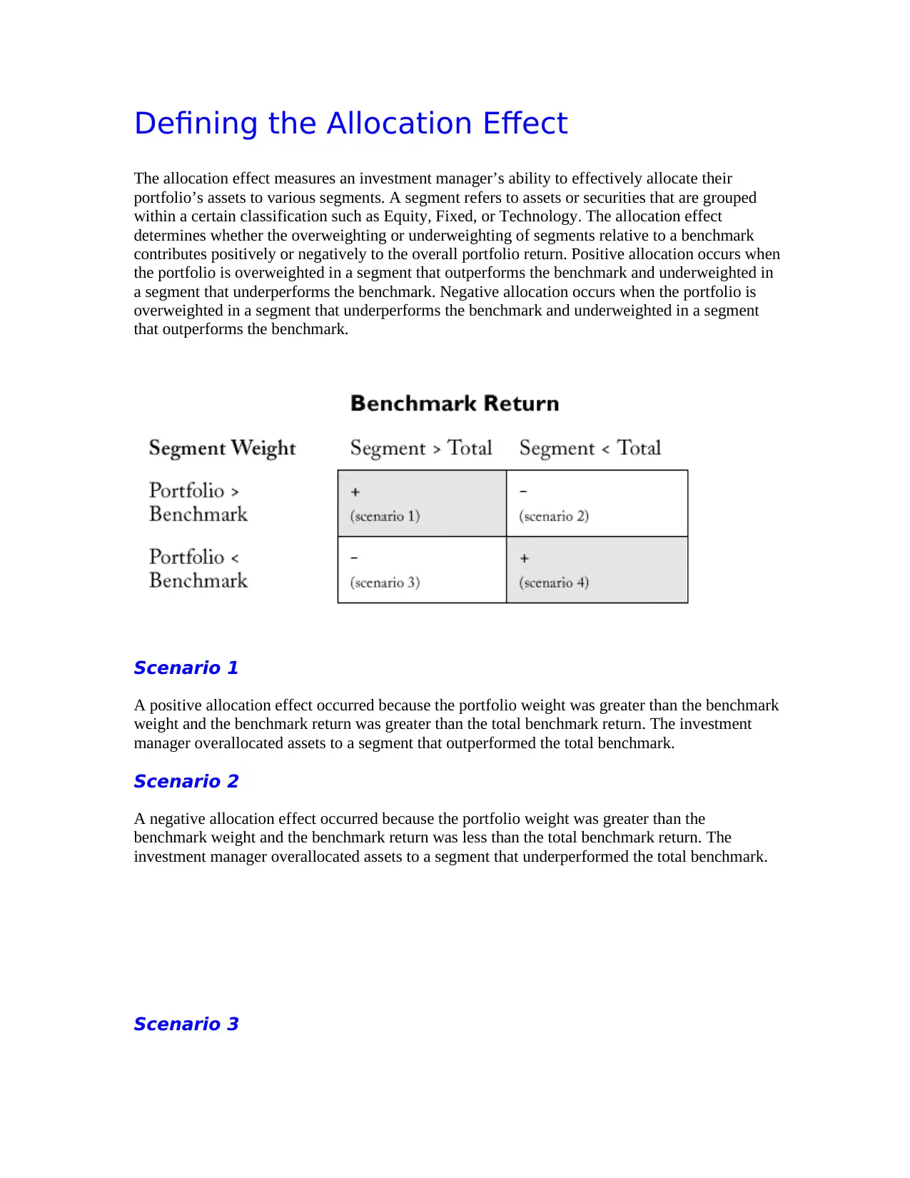
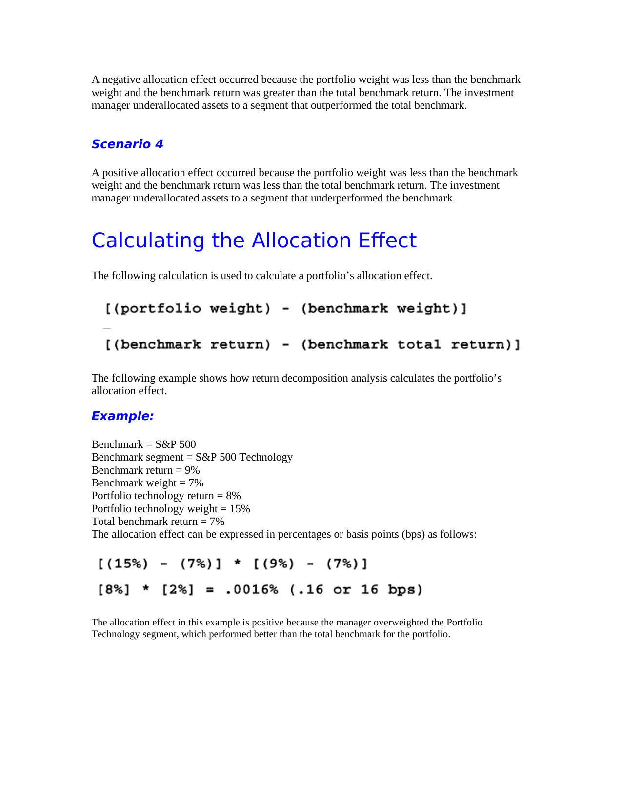
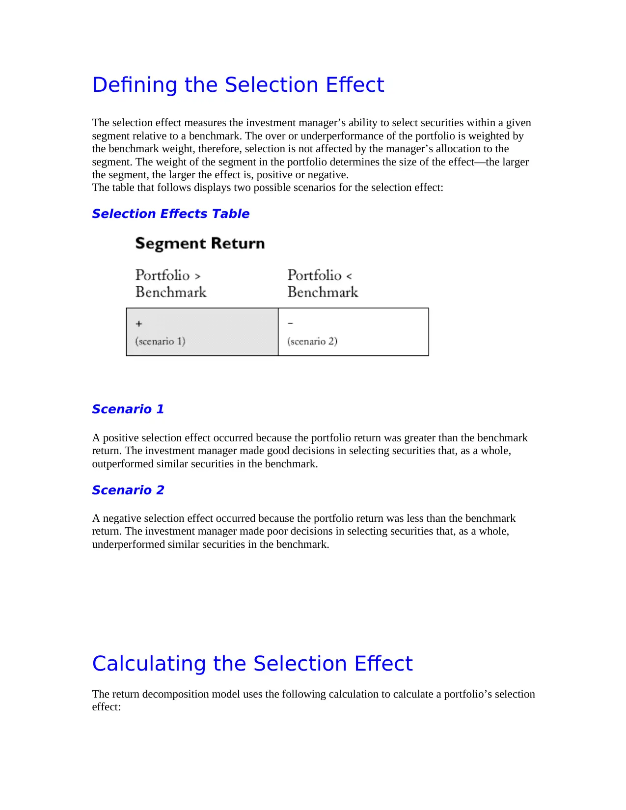
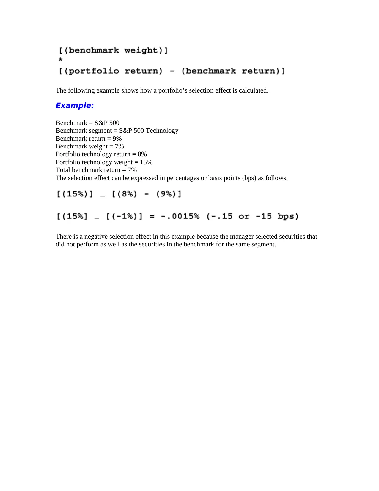
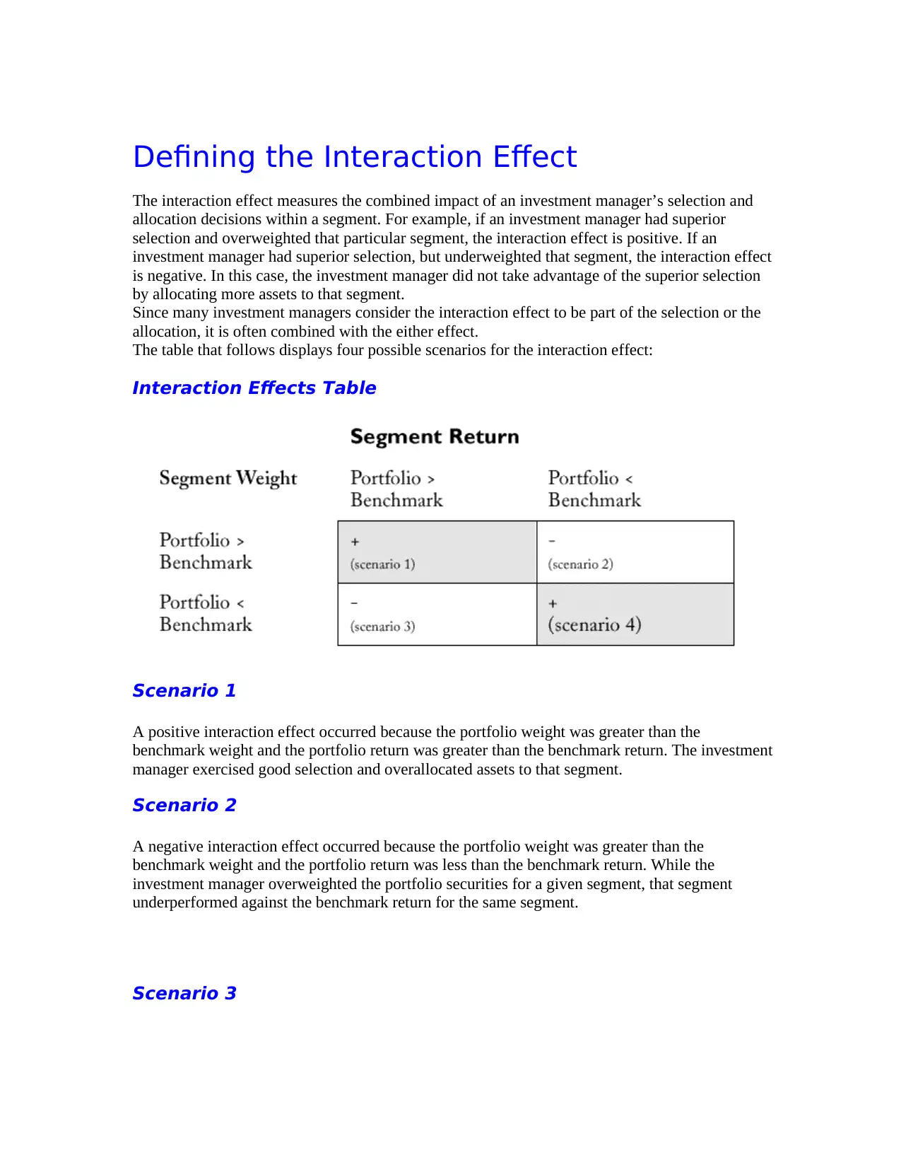
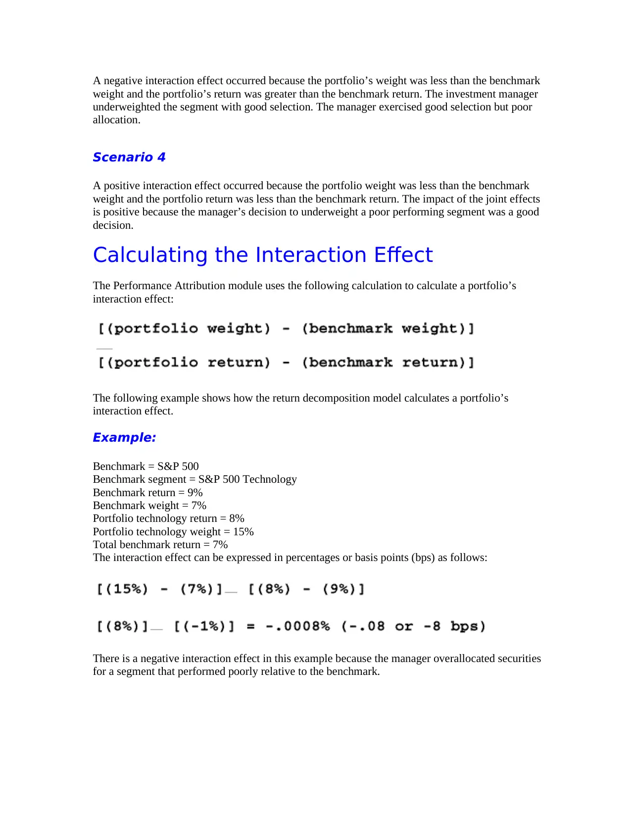
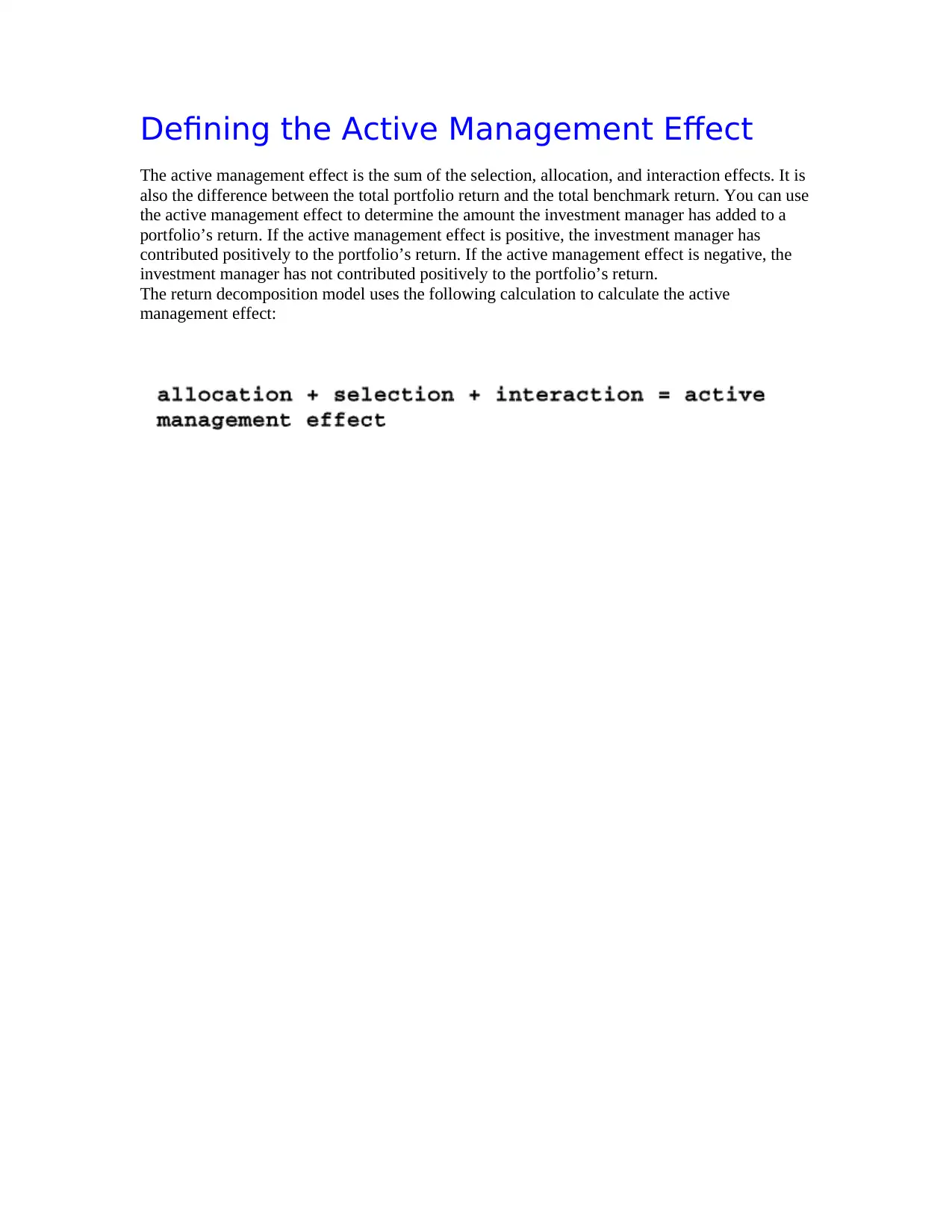
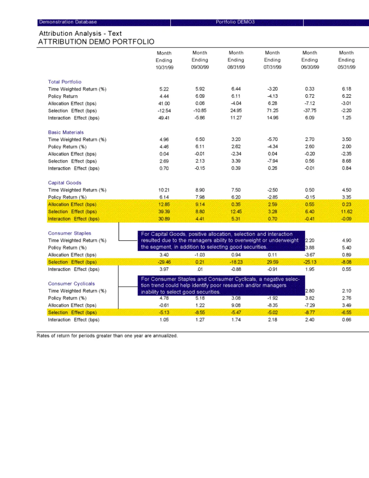
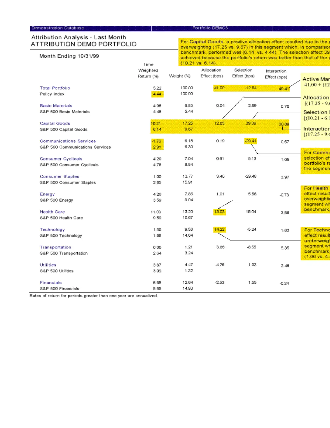
This report provides a comprehensive overview of performance attribution analysis, a crucial method for evaluating investment performance. It delves into the core concepts, including the active management effect and its components: allocation, selection, and interaction effects. The report explains how to calculate each effect using return decomposition analysis, the most widely accepted method in the investment community. The allocation effect assesses an investment manager's ability to effectively distribute assets across different segments, while the selection effect measures the manager's ability to choose successful securities within those segments. The interaction effect combines the impact of both allocation and selection decisions. The report includes scenarios and examples to illustrate how each effect contributes to overall portfolio returns, providing a practical guide for understanding and applying performance attribution in financial analysis. The report also clarifies how to determine if an investment manager has contributed positively to a portfolio’s return. Desklib offers this and other resources to help students excel in their studies.

Performance Attribution
Analysis

Preface
Performance attribution interprets how investors achieve their performance and measures the
sources of value added to a portfolio. This guide describes how returns, relative to a benchmark,
are broken down into attribution effects to determine how investors achieve performance and
measure the sources of value added to a portfolio.
About Performance Attribution
For investment managers to evaluate their job performance, they need to know how they achieved
their performance results. In particular, they need to know whether their success is the result of
their ability to effectively allocate their portfolio’s assets to various segments, their ability to
effectively select securities within a given segment or the combined effect of their selection and
allocation within a segment. Performance attribution interprets how investors achieve their
performance and measures the sources of value added to a portfolio. To determine success,
investors establish a benchmark, which they seek to outperform. Value added is the amount the
return achieves in excess of the benchmark.
Different Attribution Methods
There are generally considered to be three basic forms of attribution. These include multi-factor
analysis, style analysis and return decomposition analysis. The highlights of each are as follows:
Multi-Factor Analysis
· Attributes performance to factors such as P/E ratio, economy, bond durations, etc
· Used by academics and sophisticated firms
· More difficult to calculate
· Requires a great deal of data (economic/fundamental)
· Difficult to explain
· Not widely accepted in industry
Style Analysis
· Developed by noble laureate William Sharpe (Sharpe ratio)
· Uses portfolio rates of return to determine investment style
· Easy to calculate (requires benchmark and portfolio returns)
· Easy to explain (uses regression analysis)
· Not widely accepted in industry

Return Decomposition Analysis
· Attributes performance vs. benchmarks
· Can focus on allocation (top/down approach) or selection (bottom up approach)
· Easy to calculate ( requires benchmark and portfolio returns and weights)
· Easy to understand and explain
· Used by large portion of investment community
· Widely accepted in industry
As the return decomposition analysis is most widely used and accepted, this is the model we will
examine.
About Attribution Effects
In a return decomposition analysis model, value added to a portfolio’s return is commonly
referred to as the active management effect. The active management effect is the difference
between the total portfolio return and total benchmark return. It is also the sum of the following
investment decisions or effects:
• Allocation
• Selection
• Interaction

Defining the Allocation Effect
The allocation effect measures an investment manager’s ability to effectively allocate their
portfolio’s assets to various segments. A segment refers to assets or securities that are grouped
within a certain classification such as Equity, Fixed, or Technology. The allocation effect
determines whether the overweighting or underweighting of segments relative to a benchmark
contributes positively or negatively to the overall portfolio return. Positive allocation occurs when
the portfolio is overweighted in a segment that outperforms the benchmark and underweighted in
a segment that underperforms the benchmark. Negative allocation occurs when the portfolio is
overweighted in a segment that underperforms the benchmark and underweighted in a segment
that outperforms the benchmark.
Scenario 1
A positive allocation effect occurred because the portfolio weight was greater than the benchmark
weight and the benchmark return was greater than the total benchmark return. The investment
manager overallocated assets to a segment that outperformed the total benchmark.
Scenario 2
A negative allocation effect occurred because the portfolio weight was greater than the
benchmark weight and the benchmark return was less than the total benchmark return. The
investment manager overallocated assets to a segment that underperformed the total benchmark.
Scenario 3

A negative allocation effect occurred because the portfolio weight was less than the benchmark
weight and the benchmark return was greater than the total benchmark return. The investment
manager underallocated assets to a segment that outperformed the total benchmark.
Scenario 4
A positive allocation effect occurred because the portfolio weight was less than the benchmark
weight and the benchmark return was less than the total benchmark return. The investment
manager underallocated assets to a segment that underperformed the benchmark.
Calculating the Allocation Effect
The following calculation is used to calculate a portfolio’s allocation effect.
The following example shows how return decomposition analysis calculates the portfolio’s
allocation effect.
Example:
Benchmark = S&P 500
Benchmark segment = S&P 500 Technology
Benchmark return = 9%
Benchmark weight = 7%
Portfolio technology return = 8%
Portfolio technology weight = 15%
Total benchmark return = 7%
The allocation effect can be expressed in percentages or basis points (bps) as follows:
The allocation effect in this example is positive because the manager overweighted the Portfolio
Technology segment, which performed better than the total benchmark for the portfolio.

Defining the Selection Effect
The selection effect measures the investment manager’s ability to select securities within a given
segment relative to a benchmark. The over or underperformance of the portfolio is weighted by
the benchmark weight, therefore, selection is not affected by the manager’s allocation to the
segment. The weight of the segment in the portfolio determines the size of the effect—the larger
the segment, the larger the effect is, positive or negative.
The table that follows displays two possible scenarios for the selection effect:
Selection Effects Table
Scenario 1
A positive selection effect occurred because the portfolio return was greater than the benchmark
return. The investment manager made good decisions in selecting securities that, as a whole,
outperformed similar securities in the benchmark.
Scenario 2
A negative selection effect occurred because the portfolio return was less than the benchmark
return. The investment manager made poor decisions in selecting securities that, as a whole,
underperformed similar securities in the benchmark.
Calculating the Selection Effect
The return decomposition model uses the following calculation to calculate a portfolio’s selection
effect:

The following example shows how a portfolio’s selection effect is calculated.
Example:
Benchmark = S&P 500
Benchmark segment = S&P 500 Technology
Benchmark return = 9%
Benchmark weight = 7%
Portfolio technology return = 8%
Portfolio technology weight = 15%
Total benchmark return = 7%
The selection effect can be expressed in percentages or basis points (bps) as follows:
There is a negative selection effect in this example because the manager selected securities that
did not perform as well as the securities in the benchmark for the same segment.

Defining the Interaction Effect
The interaction effect measures the combined impact of an investment manager’s selection and
allocation decisions within a segment. For example, if an investment manager had superior
selection and overweighted that particular segment, the interaction effect is positive. If an
investment manager had superior selection, but underweighted that segment, the interaction effect
is negative. In this case, the investment manager did not take advantage of the superior selection
by allocating more assets to that segment.
Since many investment managers consider the interaction effect to be part of the selection or the
allocation, it is often combined with the either effect.
The table that follows displays four possible scenarios for the interaction effect:
Interaction Effects Table
Scenario 1
A positive interaction effect occurred because the portfolio weight was greater than the
benchmark weight and the portfolio return was greater than the benchmark return. The investment
manager exercised good selection and overallocated assets to that segment.
Scenario 2
A negative interaction effect occurred because the portfolio weight was greater than the
benchmark weight and the portfolio return was less than the benchmark return. While the
investment manager overweighted the portfolio securities for a given segment, that segment
underperformed against the benchmark return for the same segment.
Scenario 3

A negative interaction effect occurred because the portfolio’s weight was less than the benchmark
weight and the portfolio’s return was greater than the benchmark return. The investment manager
underweighted the segment with good selection. The manager exercised good selection but poor
allocation.
Scenario 4
A positive interaction effect occurred because the portfolio weight was less than the benchmark
weight and the portfolio return was less than the benchmark return. The impact of the joint effects
is positive because the manager’s decision to underweight a poor performing segment was a good
decision.
Calculating the Interaction Effect
The Performance Attribution module uses the following calculation to calculate a portfolio’s
interaction effect:
The following example shows how the return decomposition model calculates a portfolio’s
interaction effect.
Example:
Benchmark = S&P 500
Benchmark segment = S&P 500 Technology
Benchmark return = 9%
Benchmark weight = 7%
Portfolio technology return = 8%
Portfolio technology weight = 15%
Total benchmark return = 7%
The interaction effect can be expressed in percentages or basis points (bps) as follows:
There is a negative interaction effect in this example because the manager overallocated securities
for a segment that performed poorly relative to the benchmark.

Defining the Active Management Effect
The active management effect is the sum of the selection, allocation, and interaction effects. It is
also the difference between the total portfolio return and the total benchmark return. You can use
the active management effect to determine the amount the investment manager has added to a
portfolio’s return. If the active management effect is positive, the investment manager has
contributed positively to the portfolio’s return. If the active management effect is negative, the
investment manager has not contributed positively to the portfolio’s return.
The return decomposition model uses the following calculation to calculate the active
management effect: