Applying PERT Analysis: Graphing and Probability in Project Management

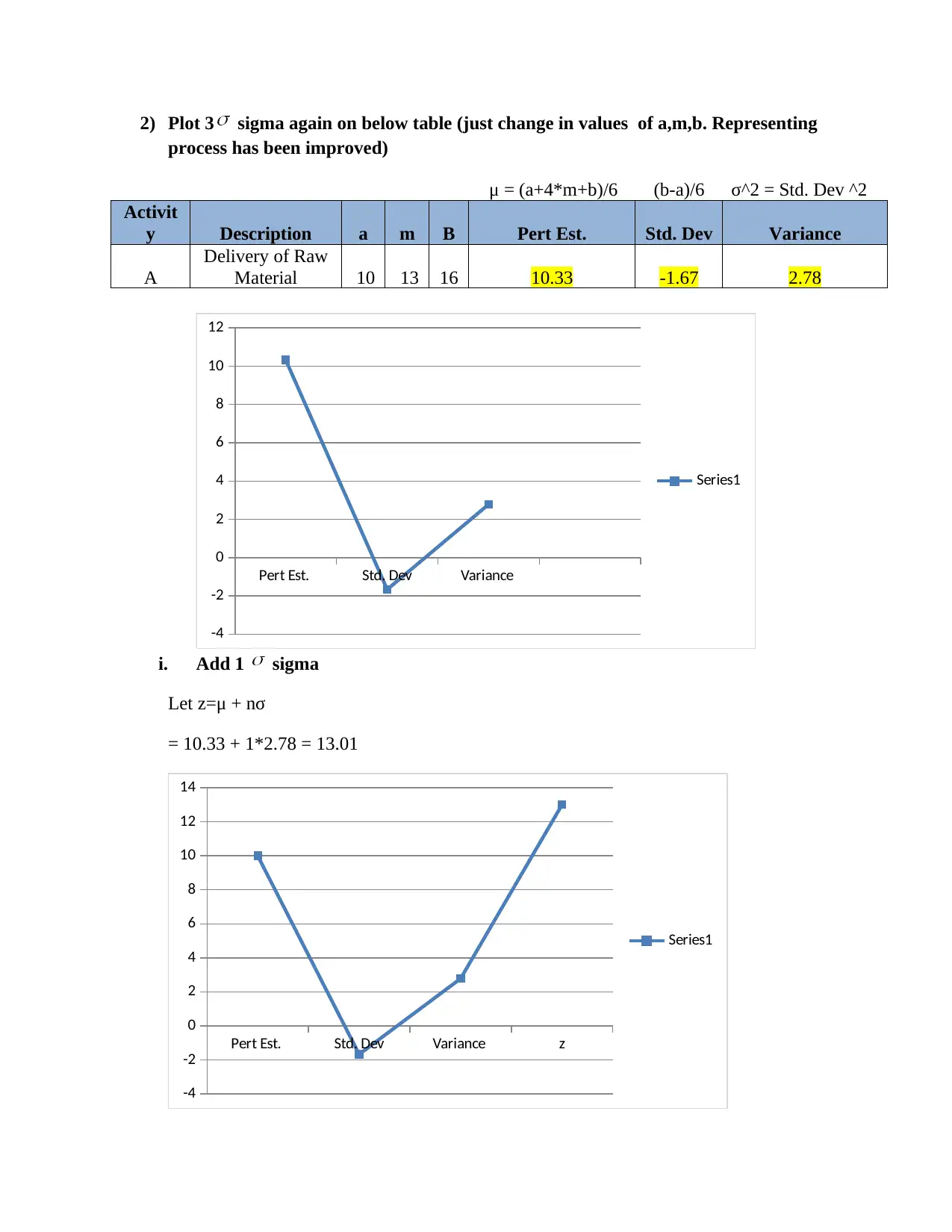
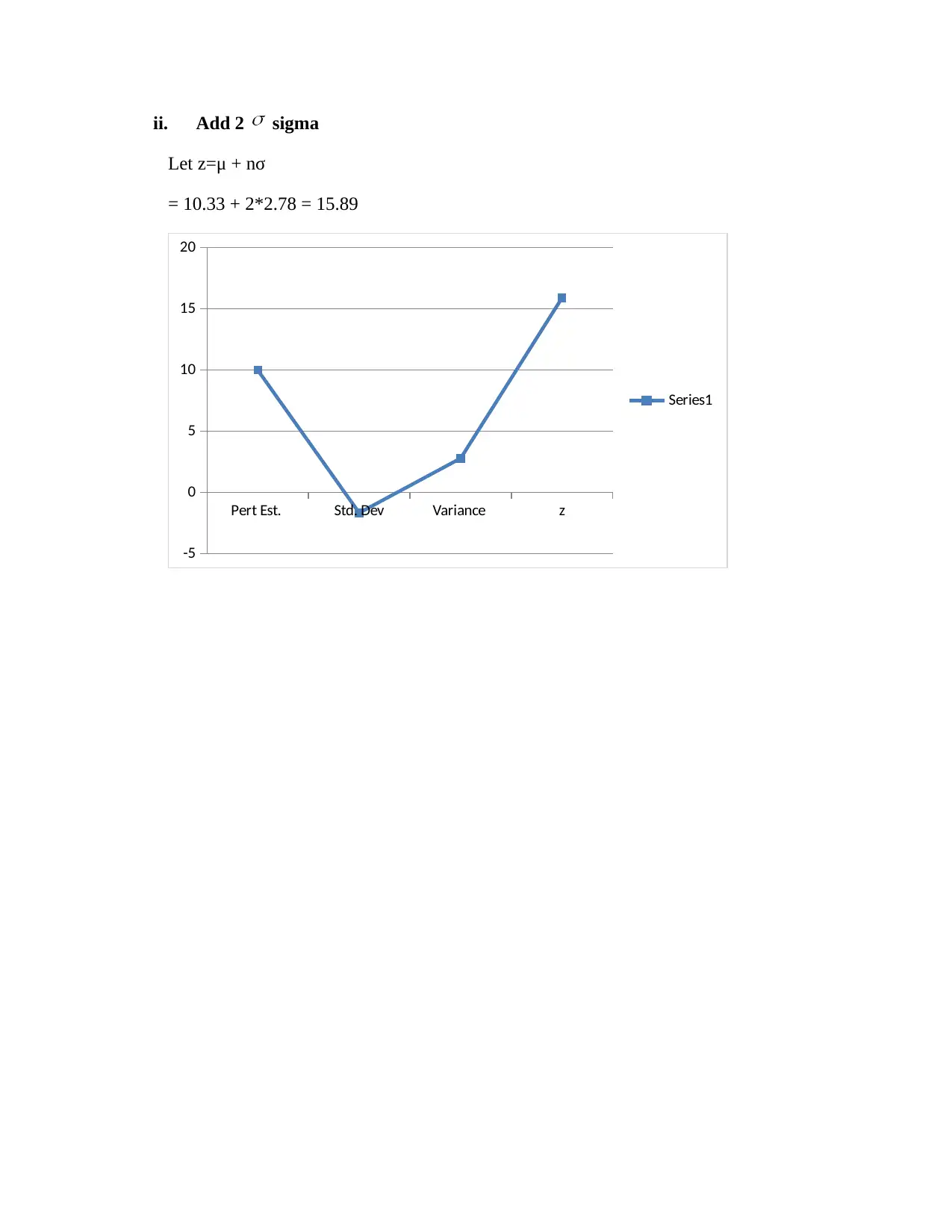
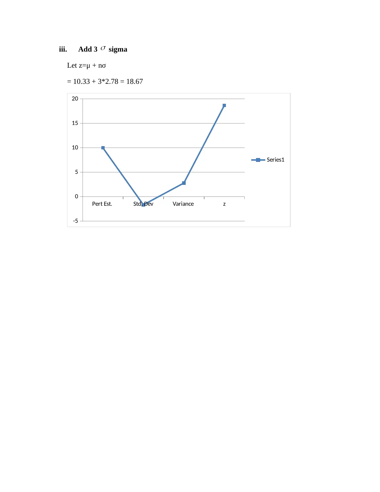
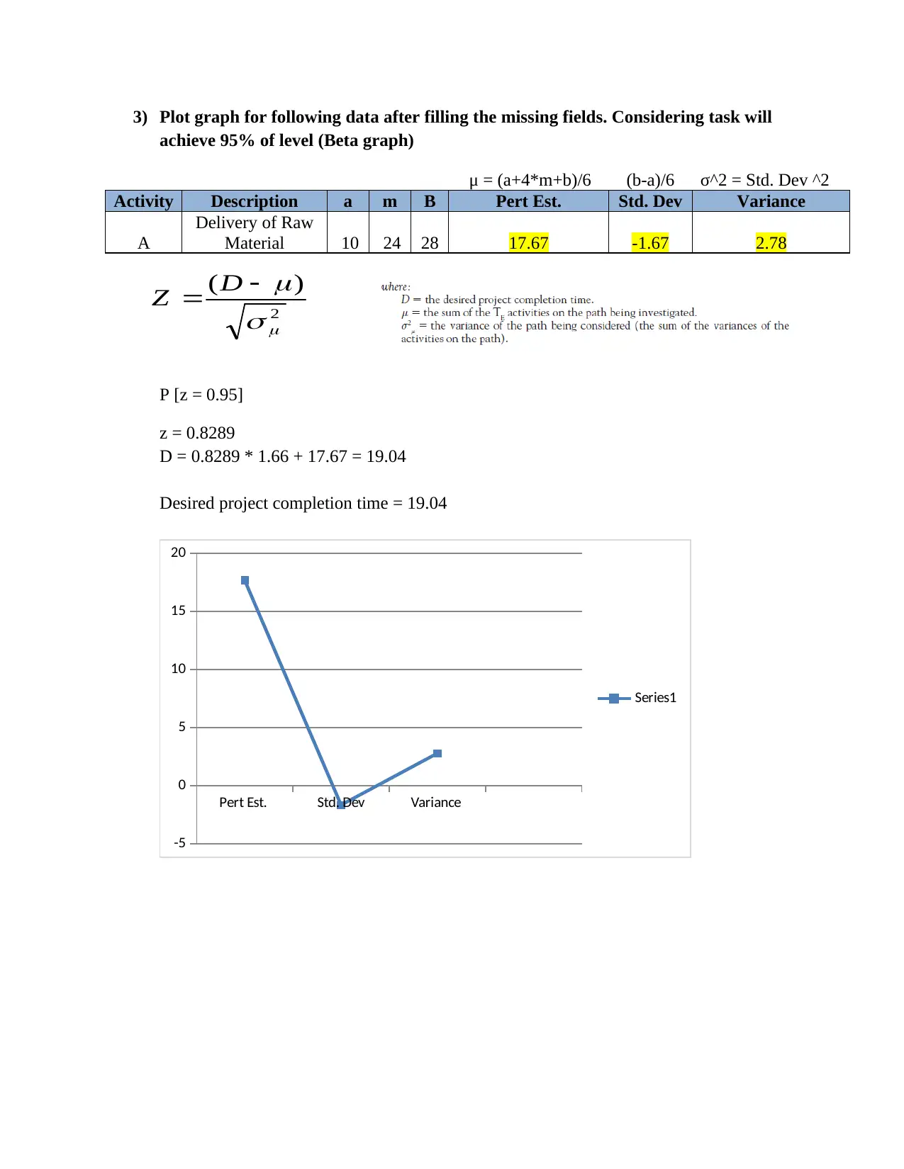
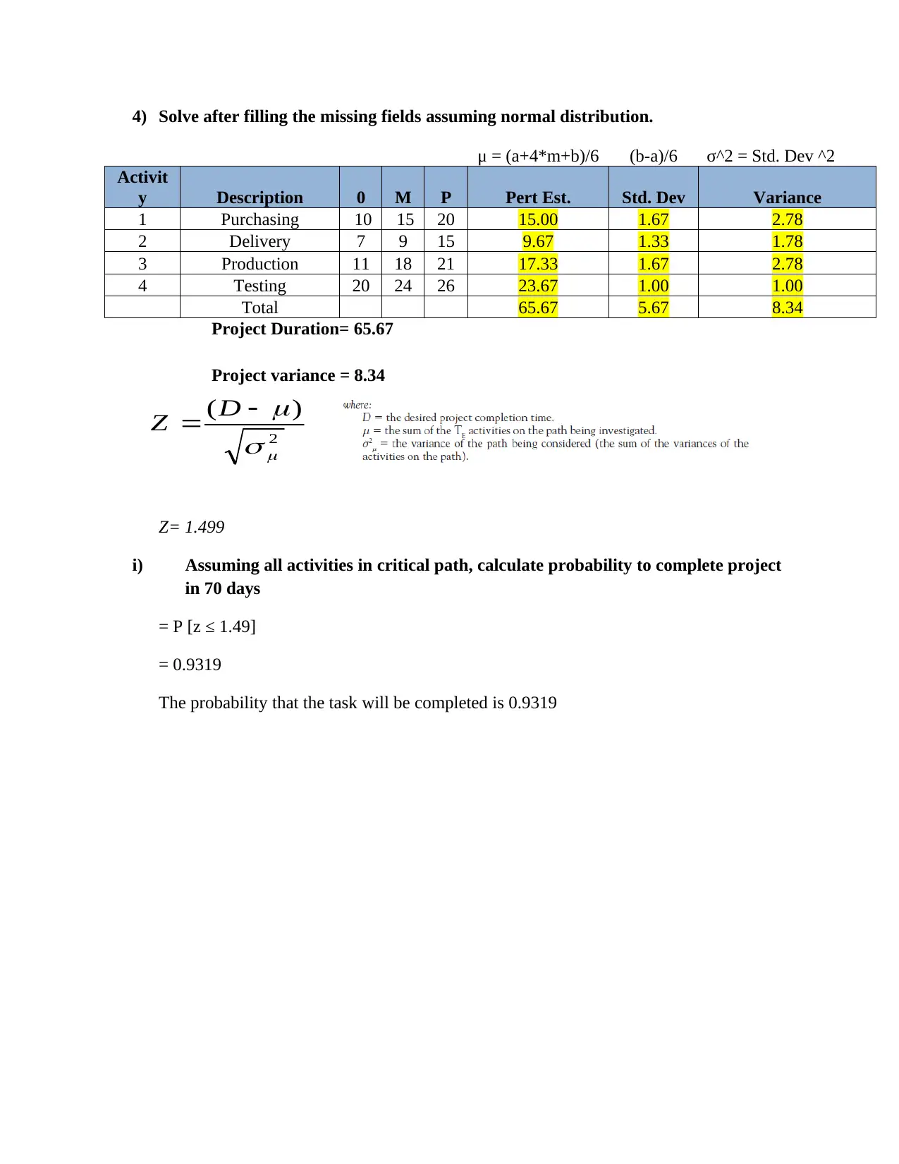
This assignment focuses on PERT (Program Evaluation and Review Technique) analysis within project management. It involves plotting graphs based on provided data, calculating estimated times and variances, and analyzing probabilities of project completion. The assignment includes scenarios involving normal distribution and improved process implementation, requiring the application of statistical concepts like standard deviation and Z-scores. Furthermore, it explores the use of Beta graphs to estimate task completion levels and solves problems related to project duration and completion probability using normal distribution assumptions. The document also includes a CPM & Float Analysis task, requiring filling a table with activities for a given organization, and then creating a network diagram with critical path. The solution provides detailed calculations and interpretations, offering insights into project scheduling and risk assessment. Desklib provides students access to this assignment solution, along with other solved papers, and study tools to aid in their learning.

Project Management
Name of Student:
Name of University:

Assignment PERT Analysis & Graphs
1) Plot graph for following normal data after filling the missing fields
μ = (a+4*m+b)/6 (b-a)/6 σ^2 = Std. Dev ^2
Activit
y Description a m B Pert Est. Std. Dev Variance
A
Delivery of Raw
Material 10 20 30 20.00 3.33 11.11
Pert Est. Std. Dev Variance
0
5
10
15
20
25
Series1

i. Consider it normal distribution & plot the graph again with 1 sigma,
Let z=μ + nσ
= 20 + 1*3.33 = 23.33
Pert Est. Std. Dev Variance z
0
5
10
15
20
25
Series1
ii. Add 2 sigma
Let z=μ + nσ
= 20 + 2*3.33 = 26.66
Pert Est. Std. Dev Variance z
0
5
10
15
20
25
30
Series1

iii. Add 3 sigma
Let z=μ + nσ
= 20 + 3*3.33 = 29.99
Pert Est. Std. Dev Variance z
0
5
10
15
20
25
30
35
Series1

2) Plot 3 sigma again on below table (just change in values of a,m,b. Representing
process has been improved)
μ = (a+4*m+b)/6 (b-a)/6 σ^2 = Std. Dev ^2
Activit
y Description a m B Pert Est. Std. Dev Variance
A
Delivery of Raw
Material 10 13 16 10.33 -1.67 2.78
Pert Est. Std. Dev Variance
-4
-2
0
2
4
6
8
10
12
Series1
i. Add 1 sigma
Let z=μ + nσ
= 10.33 + 1*2.78 = 13.01
Pert Est. Std. Dev Variance z
-4
-2
0
2
4
6
8
10
12
14
Series1

ii. Add 2 sigma
Let z=μ + nσ
= 10.33 + 2*2.78 = 15.89
Pert Est. Std. Dev Variance z
-5
0
5
10
15
20
Series1

iii. Add 3 sigma
Let z=μ + nσ
= 10.33 + 3*2.78 = 18.67
Pert Est. Std. Dev Variance z
-5
0
5
10
15
20
Series1

3) Plot graph for following data after filling the missing fields. Considering task will
achieve 95% of level (Beta graph)
μ = (a+4*m+b)/6 (b-a)/6 σ^2 = Std. Dev ^2
Activity Description a m B Pert Est. Std. Dev Variance
A
Delivery of Raw
Material 10 24 28 17.67 -1.67 2.78
P [z = 0.95]
z = 0.8289
D = 0.8289 * 1.66 + 17.67 = 19.04
Desired project completion time = 19.04
Pert Est. Std. Dev Variance
-5
0
5
10
15
20
Series1
2
)(



 D
Z

4) Solve after filling the missing fields assuming normal distribution.
μ = (a+4*m+b)/6 (b-a)/6 σ^2 = Std. Dev ^2
Activit
y Description 0 M P Pert Est. Std. Dev Variance
1 Purchasing 10 15 20 15.00 1.67 2.78
2 Delivery 7 9 15 9.67 1.33 1.78
3 Production 11 18 21 17.33 1.67 2.78
4 Testing 20 24 26 23.67 1.00 1.00
Total 65.67 5.67 8.34
Project Duration= 65.67
Project variance = 8.34
Z= 1.499
i) Assuming all activities in critical path, calculate probability to complete project
in 70 days
= P [z ≤ 1.49]
= 0.9319
The probability that the task will be completed is 0.9319
2
)(



 D
Z

References
Kerzner, H. and Kerzner, H.R., 2017. Project management: a systems approach to planning,
scheduling, and controlling. John Wiley & Sons.
Pinto, J.K., 2015. Project management: achieving competitive advantage. Prentice Hall.