Electrical Engineering: Phase Locked Loop (PLL) MATLAB Simulation

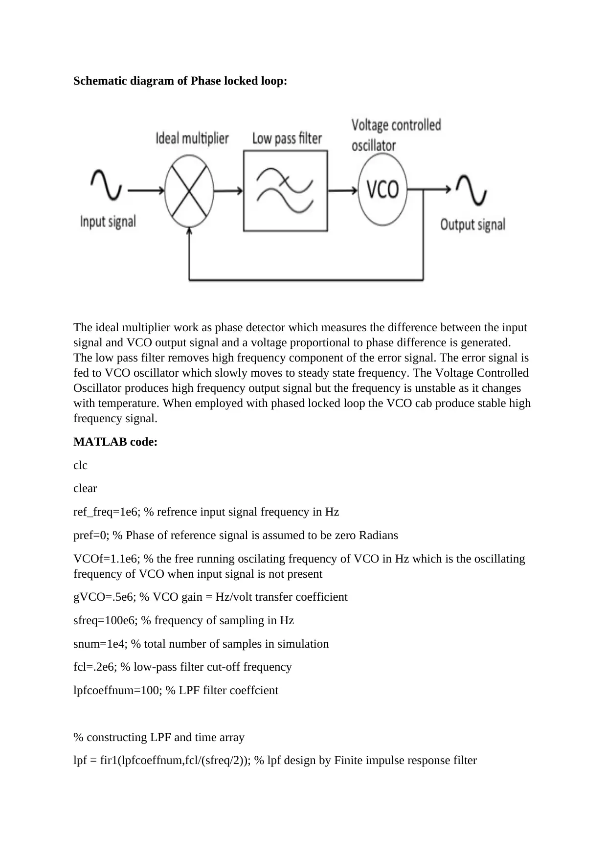
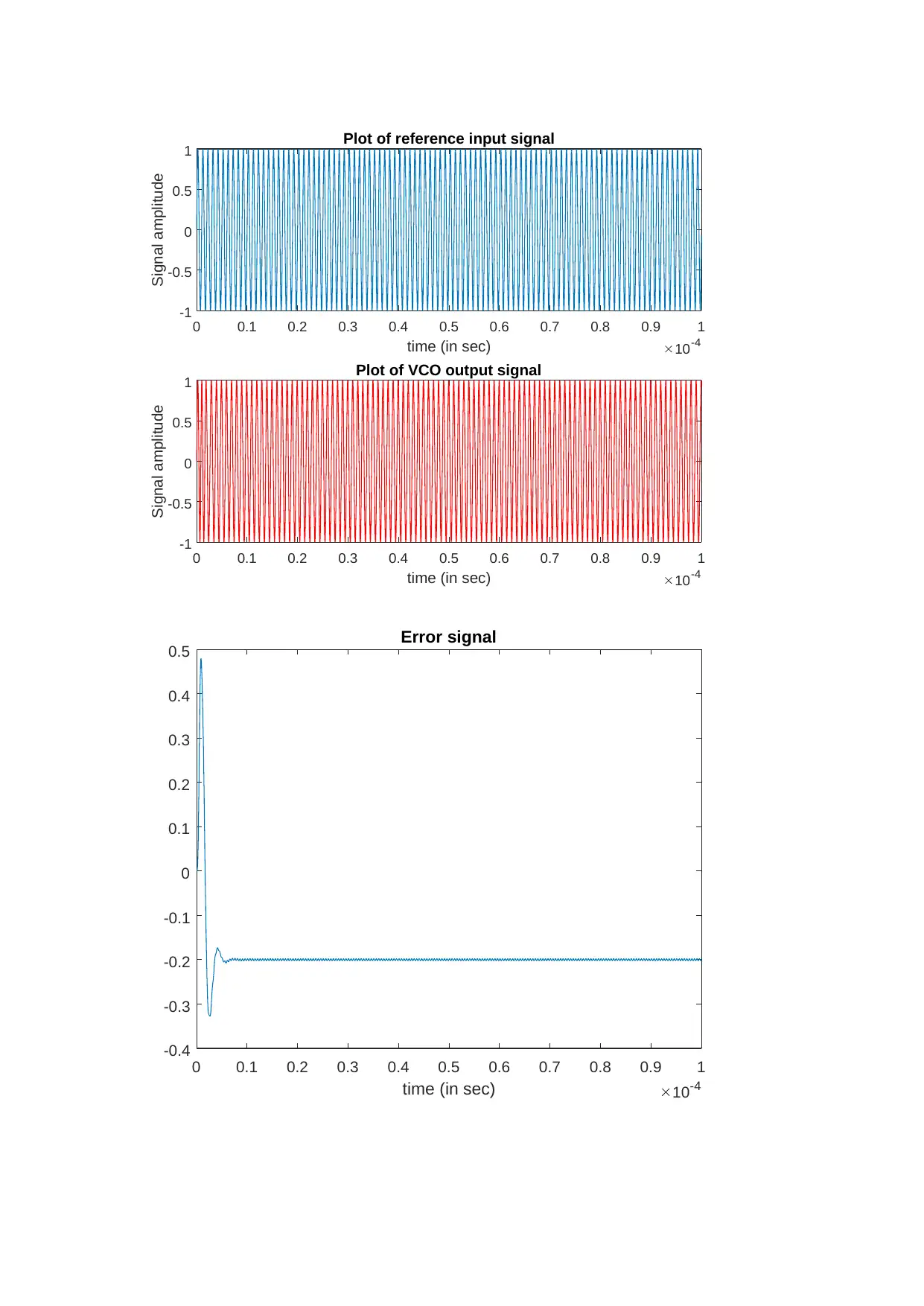
This assignment presents a detailed MATLAB simulation of a Phase Locked Loop (PLL). It begins with a schematic diagram illustrating the PLL's components: a phase detector (multiplier), a low-pass filter, and a voltage-controlled oscillator (VCO). The simulation then provides MATLAB code that implem...Read More

Schematic diagram of Phase locked loop:
The ideal multiplier work as phase detector which measures the difference between the input
signal and VCO output signal and a voltage proportional to phase difference is generated.
The low pass filter removes high frequency component of the error signal. The error signal is
fed to VCO oscillator which slowly moves to steady state frequency. The Voltage Controlled
Oscillator produces high frequency output signal but the frequency is unstable as it changes
with temperature. When employed with phased locked loop the VCO cab produce stable high
frequency signal.
MATLAB code:
clc
clear
ref_freq=1e6; % refrence input signal frequency in Hz
pref=0; % Phase of reference signal is assumed to be zero Radians
VCOf=1.1e6; % the free running oscilating frequency of VCO in Hz which is the oscillating
frequency of VCO when input signal is not present
gVCO=.5e6; % VCO gain = Hz/volt transfer coefficient
sfreq=100e6; % frequency of sampling in Hz
snum=1e4; % total number of samples in simulation
fcl=.2e6; % low-pass filter cut-off frequency
lpfcoeffnum=100; % LPF filter coeffcient
% constructing LPF and time array
lpf = fir1(lpfcoeffnum,fcl/(sfreq/2)); % lpf design by Finite impulse response filter

sp=1/sfreq;
time=0:sp:(snum-1)*sp; % time array in between 0 to 10 msec.
VCOsig=zeros(1,snum); % initializing VCO signal with zeros to increase computation speed.
phi=zeros(1,snum); % initializing VCO phase in Rads with zeros to increase computation
speed.
reference=sin(2*pi*ref_freq*time+pref); % input reference signal is assumed to be sinusoidal
with zero phase deviation
for i=2:snum
t=(i-2)*sp; % Starting time is 0 secs
mult_error(i)=reference(i)*VCOsig(i-1);% obtaining error signal by multiplication of VCO
signal and input signal
%%%Passing the error signal through LPF filter
for j=1:length(lpf)
if i-j+1>=1
errorvec(j)=mult_error(i-j+1);
else
errorvec(j)=0;
end
end
finalerror(i)=sum(errorvec.*(lpf)); % summing the error with filtered signal. This is
working of Phase detector
%%%
phi(i)=phi(i-1)+2*pi*finalerror(i)*gVCO*sp; % updating Phase of VCO in sample points
VCOsig(i)=sin(2*pi*VCOf*t+phi(i)); % VCO signal construction based on current phase
end

figure(1)
subplot(2,1,1)
plot(time,reference)
title('Plot of reference input signal')
xlabel('time (in sec)')
ylabel('Signal amplitude')
subplot(2,1,2)
plot(time,VCOsig,'r-')
title('Plot of VCO output signal')
xlabel('time (in sec)')
ylabel('Signal amplitude')
figure(2)
plot(time,finalerror)
title('Error signal')
xlabel('time (in sec)')
[peaks,locs] = findpeaks(VCOsig);
freqVCO = 1e3/(time(locs(end)) - time(locs(end - 1)));
sprintf('The frequency of the VCO output signal is %g Hz',freqVCO)
Output:
'The frequency of the VCO output signal is 1e+09 Hz'

0 0.1 0.2 0.3 0.4 0.5 0.6 0.7 0.8 0.9 1
time (in sec) 10-4
-1
-0.5
0
0.5
1
Signal amplitude
Plot of reference input signal
0 0.1 0.2 0.3 0.4 0.5 0.6 0.7 0.8 0.9 1
time (in sec) 10-4
-1
-0.5
0
0.5
1
Signal amplitude
Plot of VCO output signal
0 0.1 0.2 0.3 0.4 0.5 0.6 0.7 0.8 0.9 1
time (in sec) 10-4
-0.4
-0.3
-0.2
-0.1
0
0.1
0.2
0.3
0.4
0.5 Error signal